Network Anomography Yin Zhang yzhangcs utexas edu Joint

Network Anomography Yin Zhang yzhang@cs. utexas. edu Joint work with Zihui Ge, Albert Greenberg, Matthew Roughan Internet Measurement Conference 2005 Berkeley, CA, USA

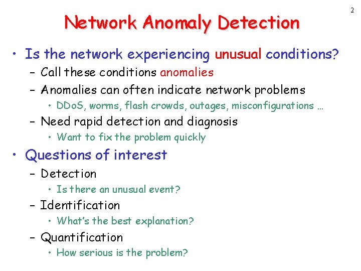
Network Anomaly Detection • Is the network experiencing unusual conditions? – Call these conditions anomalies – Anomalies can often indicate network problems • DDo. S, worms, flash crowds, outages, misconfigurations … – Need rapid detection and diagnosis • Want to fix the problem quickly • Questions of interest – Detection • Is there an unusual event? – Identification • What’s the best explanation? – Quantification • How serious is the problem? 2

3 Network Anomography • What we want B C – Volume anomalies [Lakhina 04] Significant changes in an Origin-Destination flow, i. e. , traffic matrix element • What we have – Link traffic measurements – It is difficult to measure traffic matrix directly A • Network Anomography – Infer volume anomalies from link traffic measurements

An Illustration Courtesy: Anukool Lakhina [Lakhina 04] 4

5 Anomography = Anomalies + Tomography

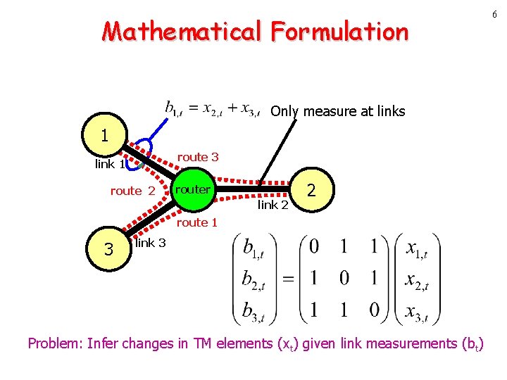
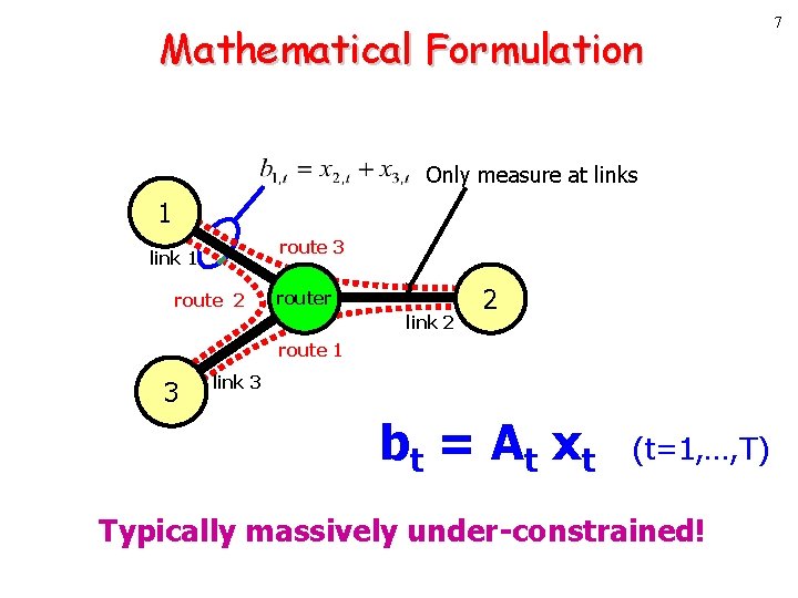
Mathematical Formulation Only measure at links 1 route 3 link 1 route 2 router link 2 2 route 1 3 link 3 Problem: Infer changes in TM elements (xt) given link measurements (bt) 6

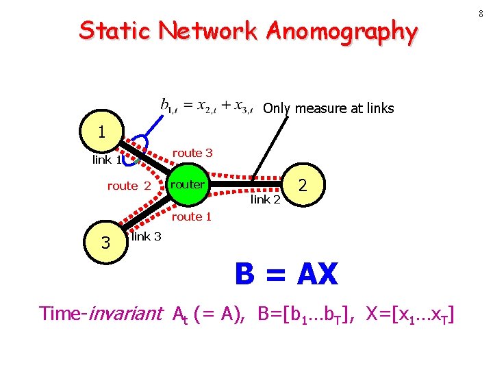
Mathematical Formulation Only measure at links 1 route 3 link 1 route 2 router link 2 2 route 1 3 link 3 b t = A t xt (t=1, …, T) Typically massively under-constrained! 7

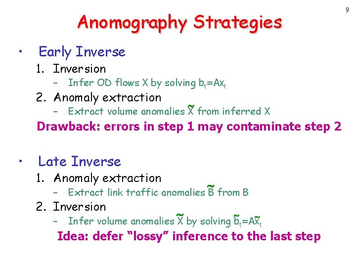
Static Network Anomography Only measure at links 1 route 3 link 1 route 2 router link 2 2 route 1 3 link 3 B = AX Time-invariant At (= A), B=[b 1…b. T], X=[x 1…x. T] 8

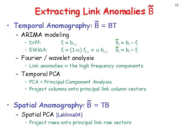
Anomography Strategies • Early Inverse 1. Inversion – Infer OD flows X by solving bt=Axt – Extract volume anomalies X from inferred X 2. Anomaly extraction Drawback: errors in step 1 may contaminate step 2 • Late Inverse 1. Anomaly extraction – Extract link traffic anomalies B from B – Infer volume anomalies X by solving bt=Ax t 2. Inversion Idea: defer “lossy” inference to the last step 9

Extracting Link Anomalies B • Temporal Anomography: B = BT – ARIMA modeling • Diff: • EWMA: ft = bt-1 ft = (1 - ) ft-1 + bt-1 – Fourier / wavelet analysis bt = bt – f t • Link anomalies = the high frequency components – Temporal PCA • PCA = Principal Component Analysis • Project columns onto principal link column vectors • Spatial Anomography: B = TB – Spatial PCA [Lakhina 04] • Project rows onto principal link row vectors 10

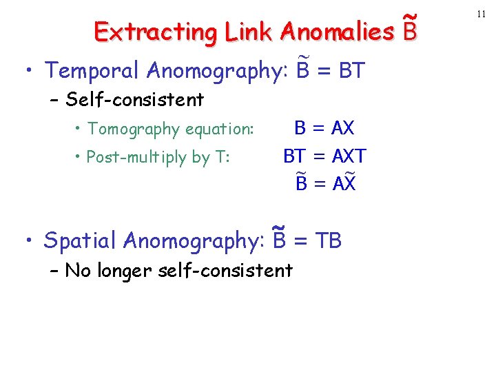
Extracting Link Anomalies B • Temporal Anomography: B = BT – Self-consistent • Tomography equation: • Post-multiply by T: B = AX BT = AXT B = AX • Spatial Anomography: B = TB – No longer self-consistent 11

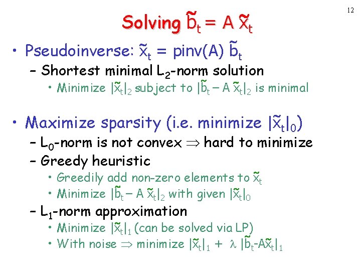
Solving bt = A xt 12 • Pseudoinverse: xt = pinv(A) bt – Shortest minimal L 2 -norm solution • Minimize |xt|2 subject to |bt – A xt|2 is minimal • Maximize sparsity (i. e. minimize |xt|0) – L 0 -norm is not convex hard to minimize – Greedy heuristic • Greedily add non-zero elements to x t • Minimize |bt – A x t|2 with given |x t|0 – L 1 -norm approximation • Minimize |x t|1 (can be solved via LP) • With noise minimize |xt|1 + |bt-Ax t|1

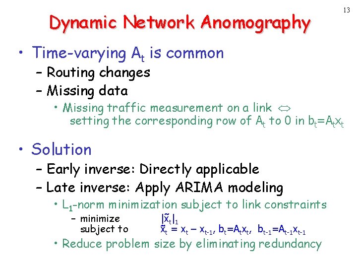
Dynamic Network Anomography 13 • Time-varying At is common – Routing changes – Missing data • Missing traffic measurement on a link setting the corresponding row of At to 0 in bt=Atxt • Solution – Early inverse: Directly applicable – Late inverse: Apply ARIMA modeling • L 1 -norm minimization subject to link constraints – minimize subject to |xt|1 x t = xt – xt-1, bt=Atxt, bt-1=At-1 xt-1 • Reduce problem size by eliminating redundancy

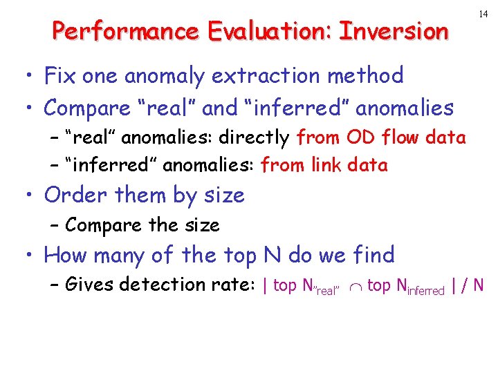
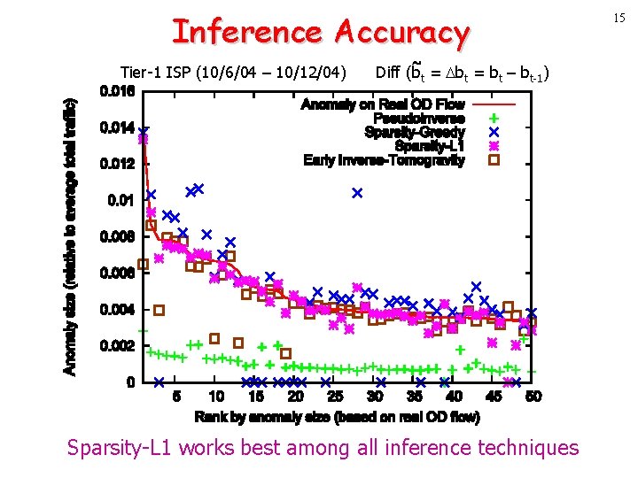
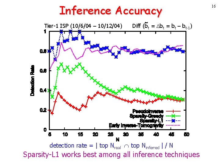
Performance Evaluation: Inversion 14 • Fix one anomaly extraction method • Compare “real” and “inferred” anomalies – “real” anomalies: directly from OD flow data – “inferred” anomalies: from link data • Order them by size – Compare the size • How many of the top N do we find – Gives detection rate: | top N”real” top Ninferred | / N

Inference Accuracy Tier-1 ISP (10/6/04 – 10/12/04) Diff (bt = bt – bt-1) Sparsity-L 1 works best among all inference techniques 15

Inference Accuracy Tier-1 ISP (10/6/04 – 10/12/04) Diff (bt = bt – bt-1) detection rate = | top Nreal top Ninferred | / N Sparsity-L 1 works best among all inference techniques 16

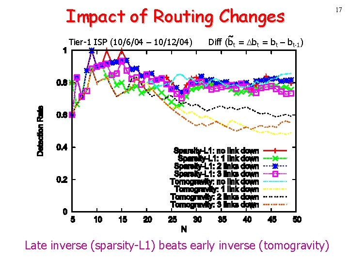
Impact of Routing Changes Tier-1 ISP (10/6/04 – 10/12/04) Diff (bt = bt – bt-1) Late inverse (sparsity-L 1) beats early inverse (tomogravity) 17

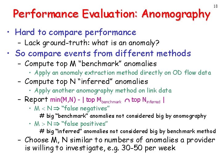
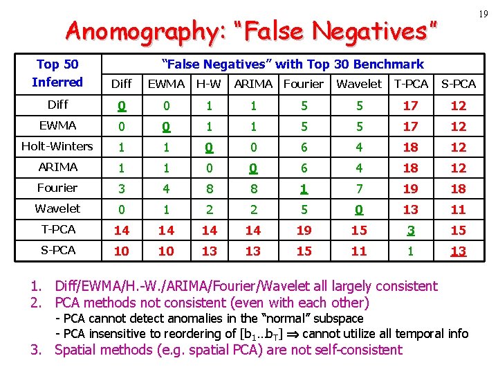
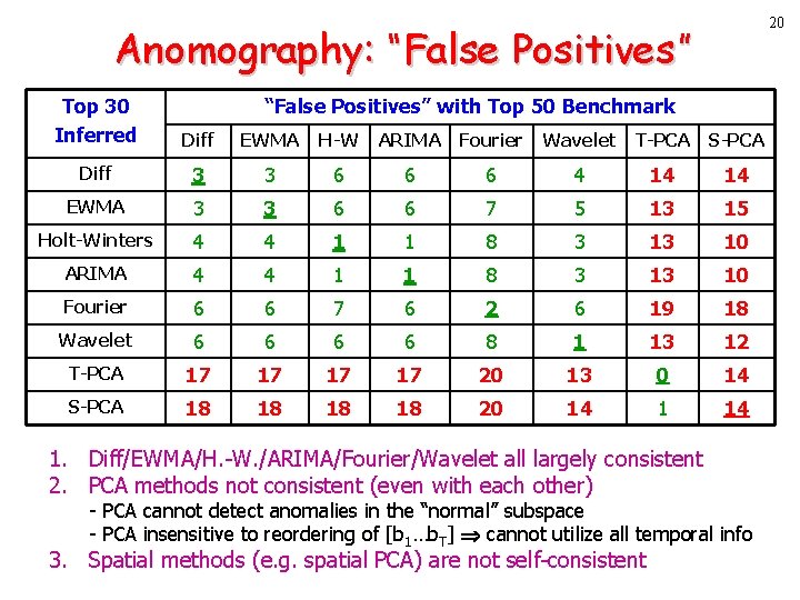
Performance Evaluation: Anomography 18 • Hard to compare performance – Lack ground-truth: what is an anomaly? • So compare events from different methods – Compute top M “benchmark” anomalies • Apply an anomaly extraction method directly on OD flow data – Compute top N “inferred” anomalies • Apply another anomography method on link data – Report min(M, N) - | top Mbenchmark top Ninferred | • M < N “false negatives” # big “benchmark” anomalies not considered big by anomography • M > N “false positives” # big “inferred” anomalies not considered big by benchmark method – Choose M, N similar to numbers of anomalies a provider is willing to investigate, e. g. 30 -50 per week

19 Anomography: “False Negatives” Top 50 Inferred “False Negatives” with Top 30 Benchmark Diff EWMA H-W ARIMA Fourier Wavelet T-PCA S-PCA Diff 0 0 1 1 5 5 17 12 EWMA 0 0 1 1 5 5 17 12 Holt-Winters 1 1 0 0 6 4 18 12 ARIMA 1 1 0 0 6 4 18 12 Fourier 3 4 8 8 1 7 19 18 Wavelet 0 1 2 2 5 0 13 11 T-PCA 14 14 19 15 3 15 S-PCA 10 10 13 13 15 11 1 13 1. Diff/EWMA/H. -W. /ARIMA/Fourier/Wavelet all largely consistent 2. PCA methods not consistent (even with each other) - PCA cannot detect anomalies in the “normal” subspace - PCA insensitive to reordering of [b 1…b. T] cannot utilize all temporal info 3. Spatial methods (e. g. spatial PCA) are not self-consistent

20 Anomography: “False Positives” Top 30 Inferred “False Positives” with Top 50 Benchmark Diff EWMA H-W ARIMA Fourier Wavelet T-PCA S-PCA Diff 3 3 6 6 6 4 14 14 EWMA 3 3 6 6 7 5 13 15 Holt-Winters 4 4 1 1 8 3 13 10 ARIMA 4 4 1 1 8 3 13 10 Fourier 6 6 7 6 2 6 19 18 Wavelet 6 6 8 1 13 12 T-PCA 17 17 20 13 0 14 S-PCA 18 18 20 14 1. Diff/EWMA/H. -W. /ARIMA/Fourier/Wavelet all largely consistent 2. PCA methods not consistent (even with each other) - PCA cannot detect anomalies in the “normal” subspace - PCA insensitive to reordering of [b 1…b. T] cannot utilize all temporal info 3. Spatial methods (e. g. spatial PCA) are not self-consistent

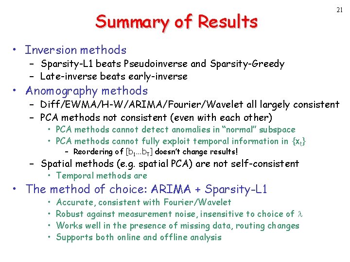
Summary of Results 21 • Inversion methods – Sparsity-L 1 beats Pseudoinverse and Sparsity-Greedy – Late-inverse beats early-inverse • Anomography methods – Diff/EWMA/H-W/ARIMA/Fourier/Wavelet all largely consistent – PCA methods not consistent (even with each other) • PCA methods cannot detect anomalies in “normal” subspace • PCA methods cannot fully exploit temporal information in {xt} – Reordering of [b 1…b. T] doesn’t change results! – Spatial methods (e. g. spatial PCA) are not self-consistent • Temporal methods are • The method of choice: ARIMA + Sparsity-L 1 • • Accurate, consistent with Fourier/Wavelet Robust against measurement noise, insensitive to choice of Works well in the presence of missing data, routing changes Supports both online and offline analysis

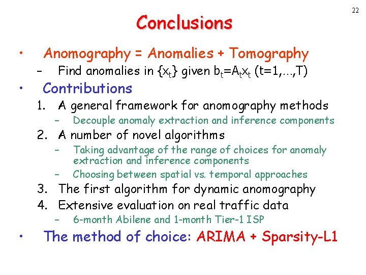
Conclusions • • – Anomography = Anomalies + Tomography Find anomalies in {xt} given bt=Atxt (t=1, …, T) Contributions 1. A general framework for anomography methods – Decouple anomaly extraction and inference components – – Taking advantage of the range of choices for anomaly extraction and inference components Choosing between spatial vs. temporal approaches – 6 -month Abilene and 1 -month Tier-1 ISP 2. A number of novel algorithms 3. The first algorithm for dynamic anomography 4. Extensive evaluation on real traffic data • The method of choice: ARIMA + Sparsity-L 1 22

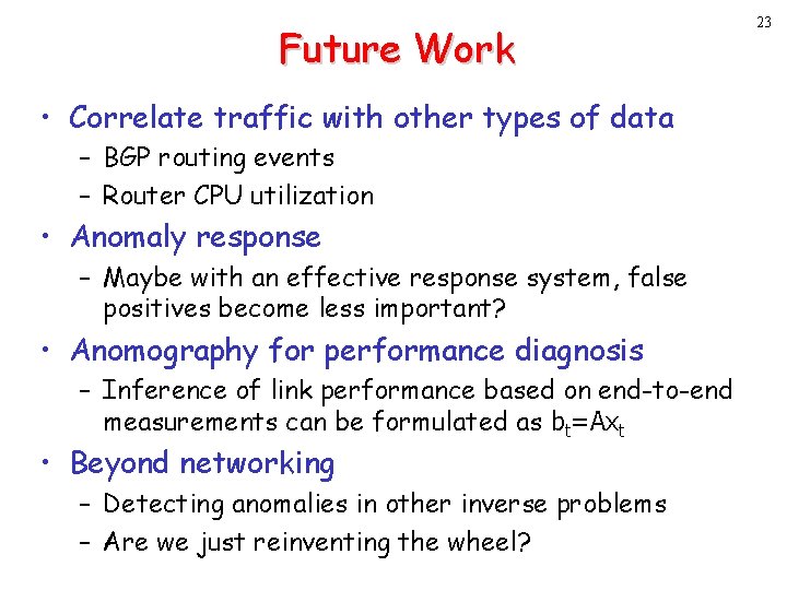
Future Work • Correlate traffic with other types of data – BGP routing events – Router CPU utilization • Anomaly response – Maybe with an effective response system, false positives become less important? • Anomography for performance diagnosis – Inference of link performance based on end-to-end measurements can be formulated as bt=Axt • Beyond networking – Detecting anomalies in other inverse problems – Are we just reinventing the wheel? 23

24 Thank you !