Online Identification of Hierarchical Heavy Hitters Yin Zhang

Online Identification of Hierarchical Heavy Hitters Yin Zhang yzhang@research. att. com Joint work with Sumeet Singh Subhabrata Sen Nick Duffield Carsten Lund Internet Measurement Conference 2004

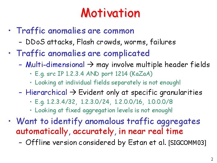
Motivation • Traffic anomalies are common – DDo. S attacks, Flash crowds, worms, failures • Traffic anomalies are complicated – Multi-dimensional may involve multiple header fields • E. g. src IP 1. 2. 3. 4 AND port 1214 (Ka. Za. A) • Looking at individual fields separately is not enough! – Hierarchical Evident only at specific granularities • E. g. 1. 2. 3. 4/32, 1. 2. 3. 0/24, 1. 2. 0. 0/16, 1. 0. 0. 0/8 • Looking at fixed aggregation levels is not enough! • Want to identify anomalous traffic aggregates automatically, accurately, in near real time – Offline version considered by Estan et al. [SIGCOMM 03] 2

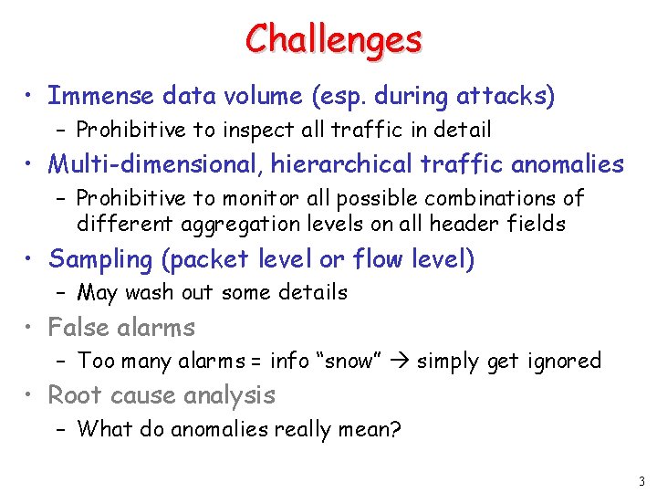
Challenges • Immense data volume (esp. during attacks) – Prohibitive to inspect all traffic in detail • Multi-dimensional, hierarchical traffic anomalies – Prohibitive to monitor all possible combinations of different aggregation levels on all header fields • Sampling (packet level or flow level) – May wash out some details • False alarms – Too many alarms = info “snow” simply get ignored • Root cause analysis – What do anomalies really mean? 3

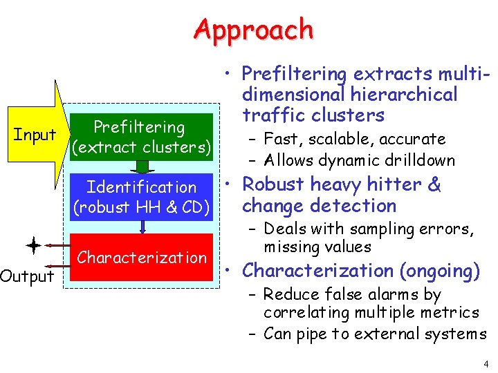
Approach Input Output Prefiltering (extract clusters) • Prefiltering extracts multidimensional hierarchical traffic clusters – Fast, scalable, accurate – Allows dynamic drilldown • Robust heavy hitter & Identification change detection (robust HH & CD) – Deals with sampling errors, missing values Characterization • Characterization (ongoing) – Reduce false alarms by correlating multiple metrics – Can pipe to external systems 4

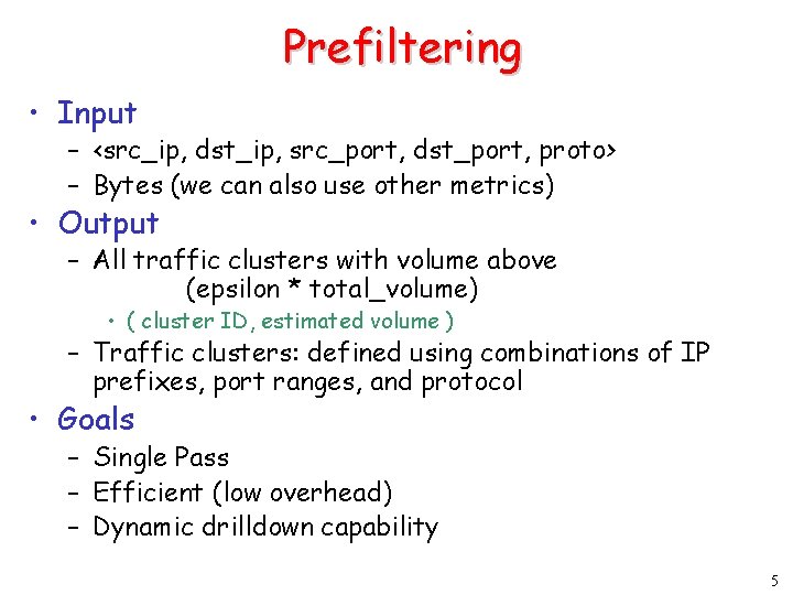
Prefiltering • Input – <src_ip, dst_ip, src_port, dst_port, proto> – Bytes (we can also use other metrics) • Output – All traffic clusters with volume above (epsilon * total_volume) • ( cluster ID, estimated volume ) – Traffic clusters: defined using combinations of IP prefixes, port ranges, and protocol • Goals – Single Pass – Efficient (low overhead) – Dynamic drilldown capability 5

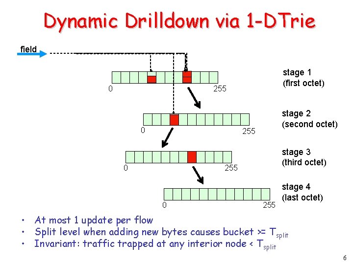
Dynamic Drilldown via 1 -DTrie field 0 stage 1 (first octet) 255 0 stage 2 (second octet) 255 0 stage 3 (third octet) 255 0 255 stage 4 (last octet) • At most 1 update per flow • Split level when adding new bytes causes bucket >= Tsplit • Invariant: traffic trapped at any interior node < Tsplit 6

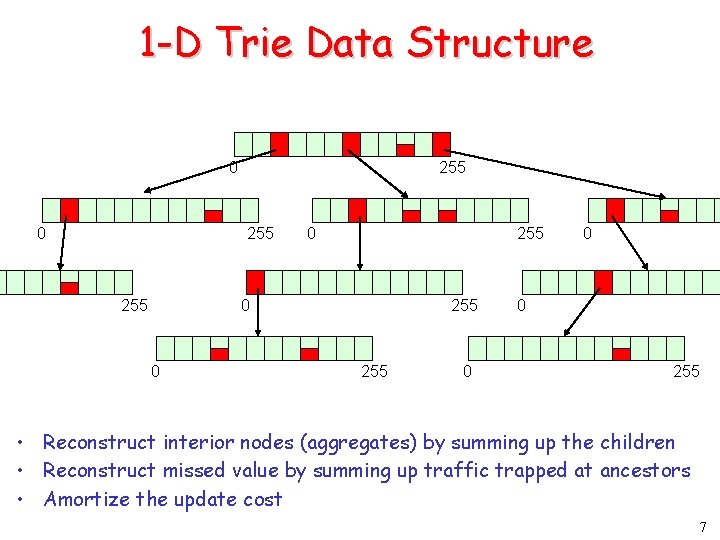
1 -D Trie Data Structure 0 0 255 0 255 0 0 0 255 • Reconstruct interior nodes (aggregates) by summing up the children • Reconstruct missed value by summing up traffic trapped at ancestors • Amortize the update cost 7

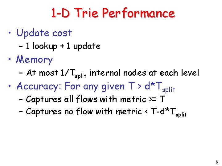
1 -D Trie Performance • Update cost – 1 lookup + 1 update • Memory – At most 1/Tsplit internal nodes at each level • Accuracy: For any given T > d*Tsplit – Captures all flows with metric >= T – Captures no flow with metric < T-d*Tsplit 8

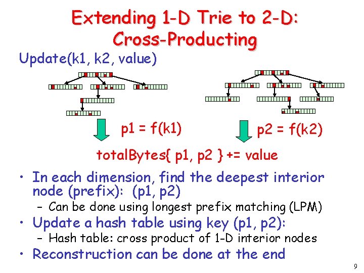
Extending 1 -D Trie to 2 -D: Cross-Producting Update(k 1, k 2, value) p 1 = f(k 1) p 2 = f(k 2) total. Bytes{ p 1, p 2 } += value • In each dimension, find the deepest interior node (prefix): (p 1, p 2) – Can be done using longest prefix matching (LPM) • Update a hash table using key (p 1, p 2): – Hash table: cross product of 1 -D interior nodes • Reconstruction can be done at the end 9

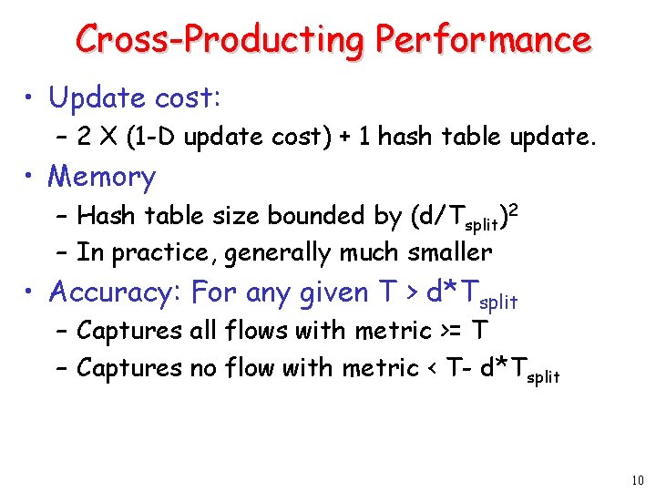
Cross-Producting Performance • Update cost: – 2 X (1 -D update cost) + 1 hash table update. • Memory – Hash table size bounded by (d/Tsplit)2 – In practice, generally much smaller • Accuracy: For any given T > d*Tsplit – Captures all flows with metric >= T – Captures no flow with metric < T- d*Tsplit 10

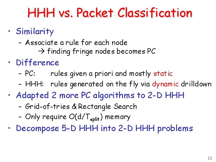
HHH vs. Packet Classification • Similarity – Associate a rule for each node finding fringe nodes becomes PC • Difference – PC: rules given a priori and mostly static – HHH: rules generated on the fly via dynamic drilldown • Adapted 2 more PC algorithms to 2 -D HHH – Grid-of-tries & Rectangle Search – Only require O(d/Tsplit) memory • Decompose 5 -D HHH into 2 -D HHH problems 11

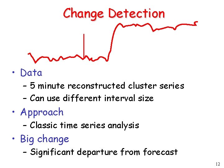
Change Detection • Data – 5 minute reconstructed cluster series – Can use different interval size • Approach – Classic time series analysis • Big change – Significant departure from forecast 12

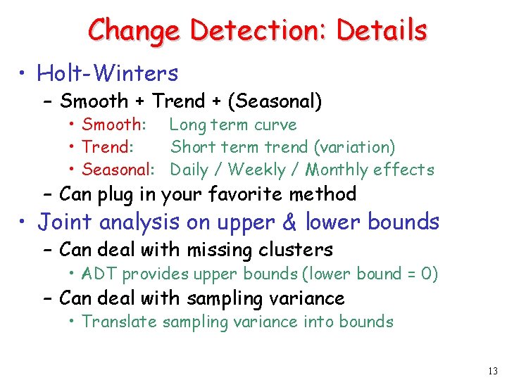
Change Detection: Details • Holt-Winters – Smooth + Trend + (Seasonal) • Smooth: Long term curve • Trend: Short term trend (variation) • Seasonal: Daily / Weekly / Monthly effects – Can plug in your favorite method • Joint analysis on upper & lower bounds – Can deal with missing clusters • ADT provides upper bounds (lower bound = 0) – Can deal with sampling variance • Translate sampling variance into bounds 13

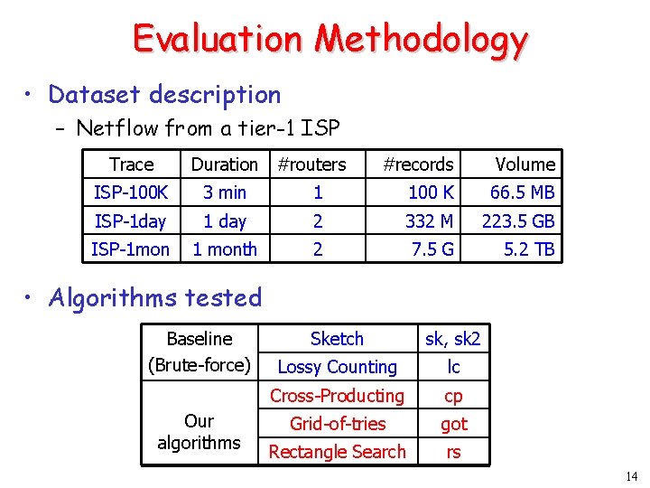
Evaluation Methodology • Dataset description – Netflow from a tier-1 ISP Trace Duration #routers #records Volume ISP-100 K 3 min 1 100 K 66. 5 MB ISP-1 day 1 day 2 332 M 223. 5 GB ISP-1 mon 1 month 2 7. 5 G 5. 2 TB • Algorithms tested Baseline (Brute-force) Our algorithms Sketch sk, sk 2 Lossy Counting lc Cross-Producting cp Grid-of-tries got Rectangle Search rs 14

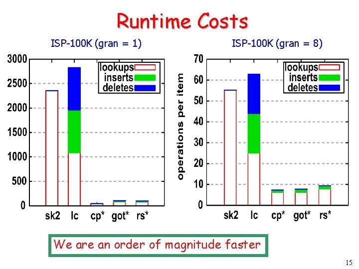
Runtime Costs ISP-100 K (gran = 1) ISP-100 K (gran = 8) We are an order of magnitude faster 15

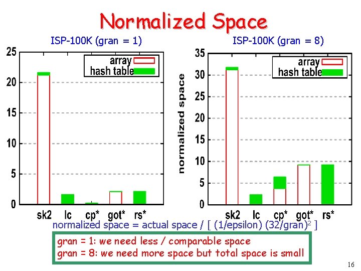
Normalized Space ISP-100 K (gran = 1) ISP-100 K (gran = 8) normalized space = actual space / [ (1/epsilon) (32/gran) 2 ] gran = 1: we need less / comparable space gran = 8: we need more space but total space is small 16

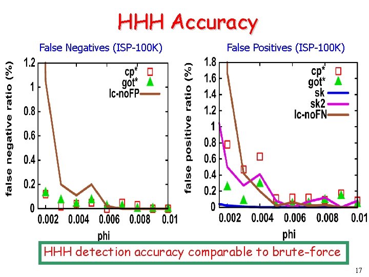
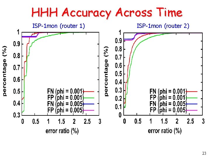
HHH Accuracy False Negatives (ISP-100 K) False Positives (ISP-100 K) HHH detection accuracy comparable to brute-force 17

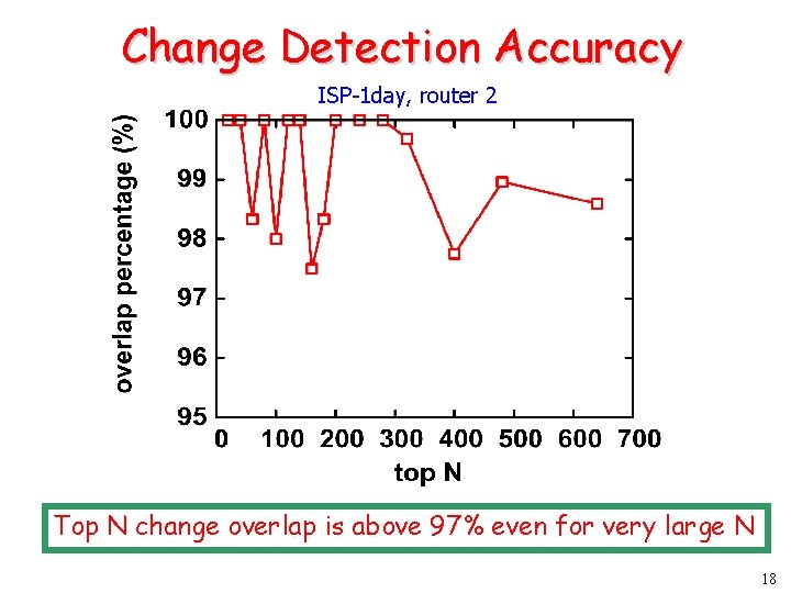
Change Detection Accuracy ISP-1 day, router 2 Top N change overlap is above 97% even for very large N 18

Effects of Sampling ISP-1 day, router 2 Accuracy above 90% with 90% data reduction 19

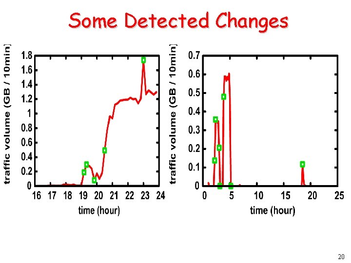
Some Detected Changes 20

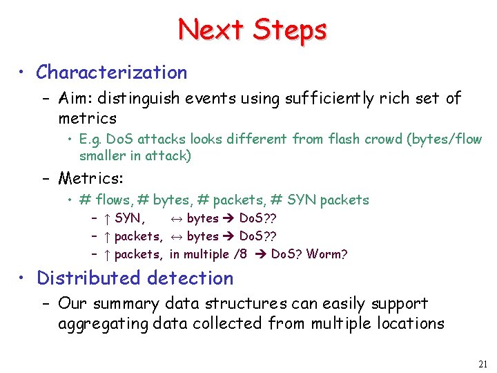
Next Steps • Characterization – Aim: distinguish events using sufficiently rich set of metrics • E. g. Do. S attacks looks different from flash crowd (bytes/flow smaller in attack) – Metrics: • # flows, # bytes, # packets, # SYN packets – ↑ SYN, ↔ bytes Do. S? ? – ↑ packets, in multiple /8 Do. S? Worm? • Distributed detection – Our summary data structures can easily support aggregating data collected from multiple locations 21

Thank you! 22

HHH Accuracy Across Time ISP-1 mon (router 1) ISP-1 mon (router 2) 23