Multivariate Methods in Particle Physics Today and Tomorrow

Multivariate Methods in Particle Physics Today and Tomorrow Harrison B. Prosper Florida State University 5 November, 2008 ACAT 08, Erice, Sicily Multivariate Methods Harrison B. Prosper ACAT 08

Outline h Introduction h Multivariate Methods h. In Theory h. In Practice h Outstanding Issues h Summary Multivariate Methods Harrison B. Prosper ACAT 08 2

Introduction Multivariate methods can be useful in: h. Classification h. Function approximation h. Probability density estimation h. Data compression h. Variable selection h. Optimization h. Model comparison Multivariate Methods Harrison B. Prosper ACAT 08 3

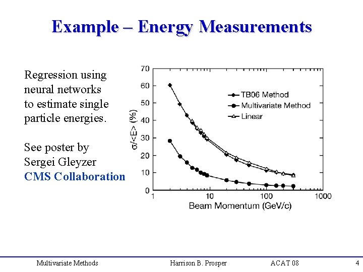
Example – Energy Measurements Regression using neural networks to estimate single particle energies. See poster by Sergei Gleyzer CMS Collaboration Multivariate Methods Harrison B. Prosper ACAT 08 4

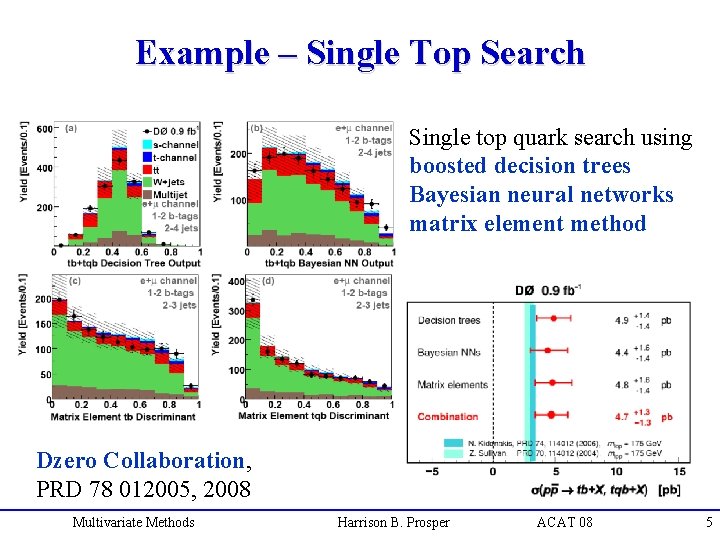
Example – Single Top Search Single top quark search using boosted decision trees Bayesian neural networks matrix element method Dzero Collaboration, PRD 78 012005, 2008 Multivariate Methods Harrison B. Prosper ACAT 08 5

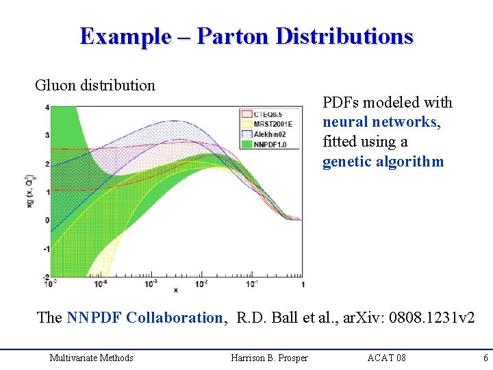
Example – Parton Distributions Gluon distribution PDFs modeled with neural networks, fitted using a genetic algorithm The NNPDF Collaboration, R. D. Ball et al. , ar. Xiv: 0808. 1231 v 2 Multivariate Methods Harrison B. Prosper ACAT 08 6

Multivariate Methods: In Theory Multivariate Methods Harrison B. Prosper ACAT 08

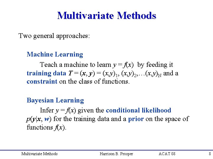
Multivariate Methods Two general approaches: Machine Learning Teach a machine to learn y = f(x) by feeding it training data T = (x, y)1, (x, y)2, …(x, y)N and a constraint on the class of functions. Bayesian Learning Infer y = f(x) given the conditional likelihood p(y|x, w) for the training data and a prior on the space of functions f(x). Multivariate Methods Harrison B. Prosper ACAT 08 8

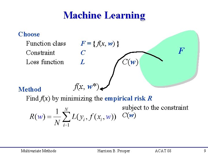
Machine Learning Choose Function class Constraint Loss function F = { f(x, w) } C L C(w) F f(x, w*) Method Find f(x) by minimizing the empirical risk R subject to the constraint C(w) Multivariate Methods Harrison B. Prosper ACAT 08 9

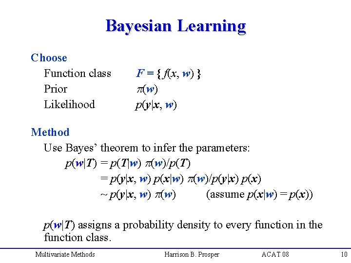
Bayesian Learning Choose Function class Prior Likelihood F = { f(x, w) } p(w) p(y|x, w) Method Use Bayes’ theorem to infer the parameters: p(w|T) = p(T|w) p(w)/p(T) = p(y|x, w) p(x|w) p(w)/p(y|x) p(x) ~ p(y|x, w) p(w) (assume p(x|w) = p(x)) p(w|T) assigns a probability density to every function in the function class. Multivariate Methods Harrison B. Prosper ACAT 08 10

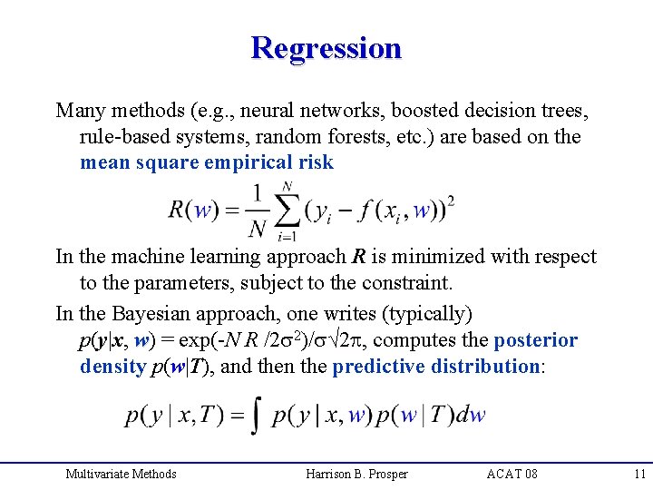
Regression Many methods (e. g. , neural networks, boosted decision trees, rule-based systems, random forests, etc. ) are based on the mean square empirical risk In the machine learning approach R is minimized with respect to the parameters, subject to the constraint. In the Bayesian approach, one writes (typically) p(y|x, w) = exp(-N R /2 s 2)/s√ 2 p, computes the posterior density p(w|T), and then the predictive distribution: Multivariate Methods Harrison B. Prosper ACAT 08 11

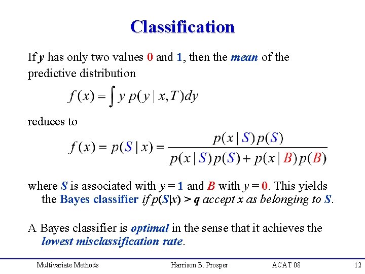
Classification If y has only two values 0 and 1, then the mean of the predictive distribution reduces to where S is associated with y = 1 and B with y = 0. This yields the Bayes classifier if p(S|x) > q accept x as belonging to S. A Bayes classifier is optimal in the sense that it achieves the lowest misclassification rate. Multivariate Methods Harrison B. Prosper ACAT 08 12

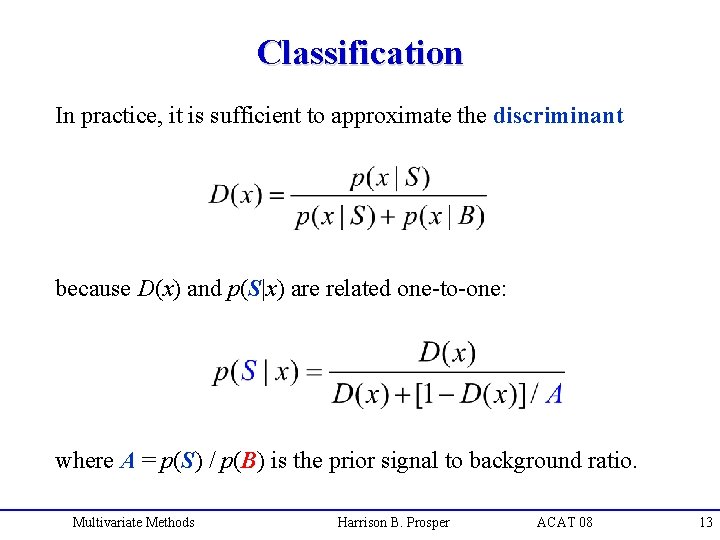
Classification In practice, it is sufficient to approximate the discriminant because D(x) and p(S|x) are related one-to-one: where A = p(S) / p(B) is the prior signal to background ratio. Multivariate Methods Harrison B. Prosper ACAT 08 13

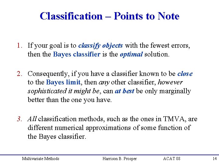
Classification – Points to Note 1. If your goal is to classify objects with the fewest errors, then the Bayes classifier is the optimal solution. 2. Consequently, if you have a classifier known to be close to the Bayes limit, then any other classifier, however sophisticated it might be, can at best be only marginally better than the one you have. 3. All classification methods, such as the ones in TMVA, are different numerical approximations of some function of the Bayes classifier. Multivariate Methods Harrison B. Prosper ACAT 08 14

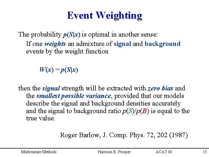
Event Weighting The probability p(S|x) is optimal in another sense: If one weights an admixture of signal and background events by the weight function W(x) = p(S|x) then the signal strength will be extracted with zero bias and the smallest possible variance, provided that our models describe the signal and background densities accurately and the signal to background ratio p(S)/p(B) is equal to the true value. Roger Barlow, J. Comp. Phys. 72, 202 (1987) Multivariate Methods Harrison B. Prosper ACAT 08 15

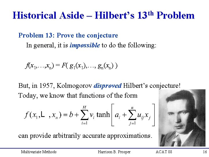
Historical Aside – Hilbert’s 13 th Problem 13: Prove the conjecture In general, it is impossible to do the following: f(x 1, …, xn) = F( g 1(x 1), …, gn(xn) ) But, in 1957, Kolmogorov disproved Hilbert’s conjecture! Today, we know that functions of the form can provide arbitrarily accurate approximations. Multivariate Methods Harrison B. Prosper ACAT 08 16

Multivariate Methods: In Practice Multivariate Methods Harrison B. Prosper ACAT 08

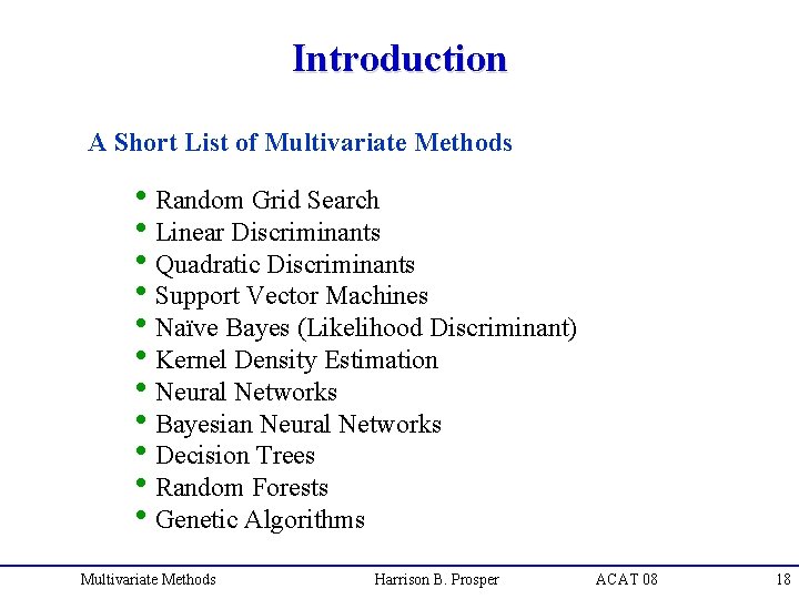
Introduction A Short List of Multivariate Methods h. Random Grid Search h. Linear Discriminants h. Quadratic Discriminants h. Support Vector Machines h. Naïve Bayes (Likelihood Discriminant) h. Kernel Density Estimation h. Neural Networks h. Bayesian Neural Networks h. Decision Trees h. Random Forests h. Genetic Algorithms Multivariate Methods Harrison B. Prosper ACAT 08 18

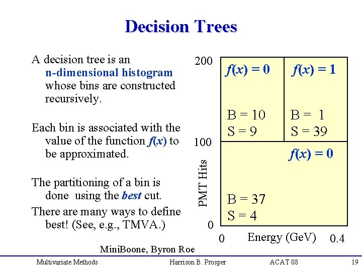
Decision Trees Each bin is associated with the value of the function f(x) to be approximated. 200 100 The partitioning of a bin is done using the best cut. There are many ways to define best! (See, e. g. , TMVA. ) Mini. Boone, Byron Roe Multivariate Methods 0 f(x) = 1 B = 10 S=9 B= 1 S = 39 f(x) = 0 PMT Hits A decision tree is an n-dimensional histogram whose bins are constructed recursively. B = 37 S=4 0 Harrison B. Prosper Energy (Ge. V) ACAT 08 0. 4 19

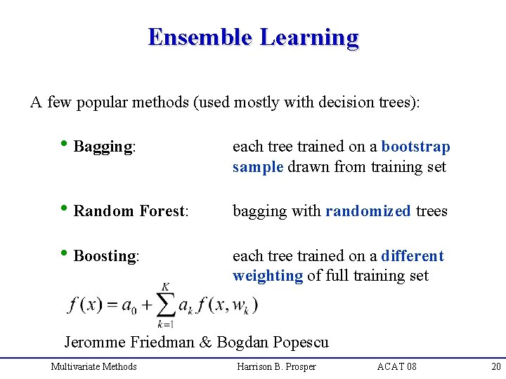
Ensemble Learning A few popular methods (used mostly with decision trees): h. Bagging: each tree trained on a bootstrap sample drawn from training set h. Random Forest: bagging with randomized trees h. Boosting: each tree trained on a different weighting of full training set Jeromme Friedman & Bogdan Popescu Multivariate Methods Harrison B. Prosper ACAT 08 20

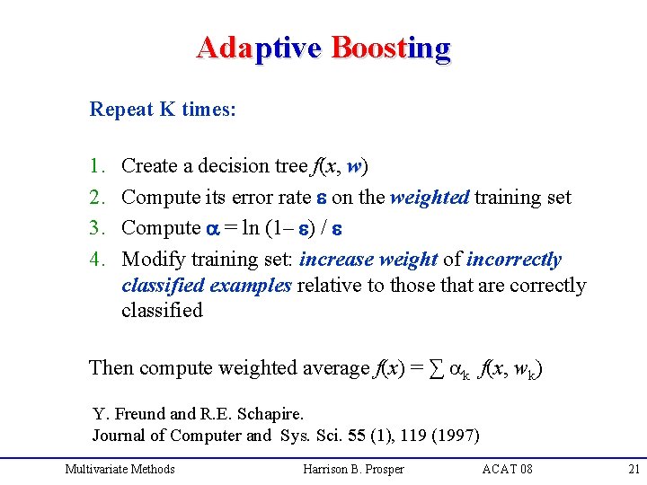
Adaptive Boosting Repeat K times: 1. 2. 3. 4. Create a decision tree f(x, w) Compute its error rate e on the weighted training set Compute a = ln (1– e) / e Modify training set: increase weight of incorrectly classified examples relative to those that are correctly classified Then compute weighted average f(x) = ∑ ak f(x, wk) Y. Freund and R. E. Schapire. Journal of Computer and Sys. Sci. 55 (1), 119 (1997) Multivariate Methods Harrison B. Prosper ACAT 08 21

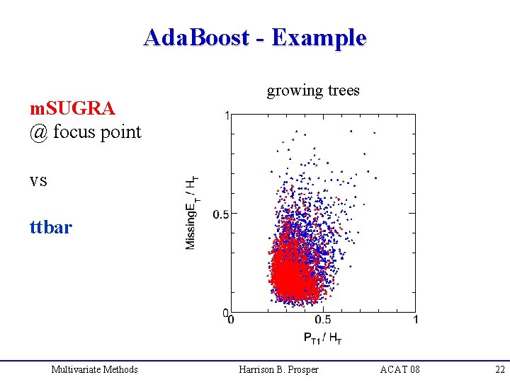
Ada. Boost - Example m. SUGRA @ focus point growing trees vs ttbar Multivariate Methods Harrison B. Prosper ACAT 08 22

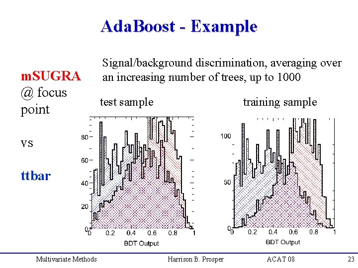
Ada. Boost - Example m. SUGRA @ focus point Signal/background discrimination, averaging over an increasing number of trees, up to 1000 test sample training sample vs ttbar Multivariate Methods Harrison B. Prosper ACAT 08 23

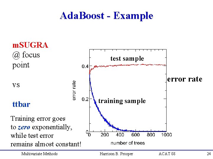
Ada. Boost - Example m. SUGRA @ focus point test sample error rate vs ttbar training sample Training error goes to zero exponentially, while test error remains almost constant! Multivariate Methods Harrison B. Prosper ACAT 08 24

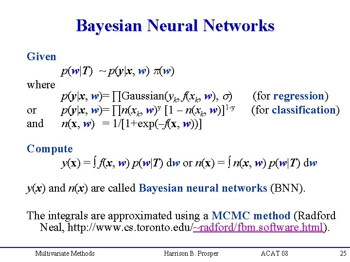
Bayesian Neural Networks Given where or and p(w|T) ~ p(y|x, w)= ∏Gaussian(yk, f(xk, w), s) p(y|x, w)= ∏n(xk, w)y [1 – n(xk, w)]1 -y n(x, w) = 1/[1+exp(–f(x, w))] (for regression) (for classification) Compute y(x) = ∫ f(x, w) p(w|T) dw or n(x) = ∫ n(x, w) p(w|T) dw y(x) and n(x) are called Bayesian neural networks (BNN). The integrals are approximated using a MCMC method (Radford Neal, http: //www. cs. toronto. edu/~radford/fbm. software. html). Multivariate Methods Harrison B. Prosper ACAT 08 25

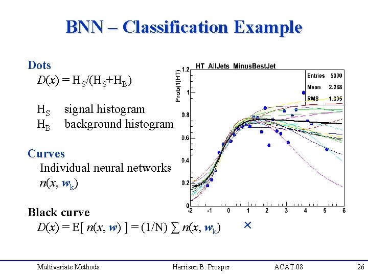
BNN – Classification Example Dots D(x) = HS/(HS+HB) HS HB signal histogram background histogram Curves Individual neural networks n(x, wk) Black curve D(x) = E[ n(x, w) ] = (1/N) ∑ n(x, wk) Multivariate Methods Harrison B. Prosper x ACAT 08 26

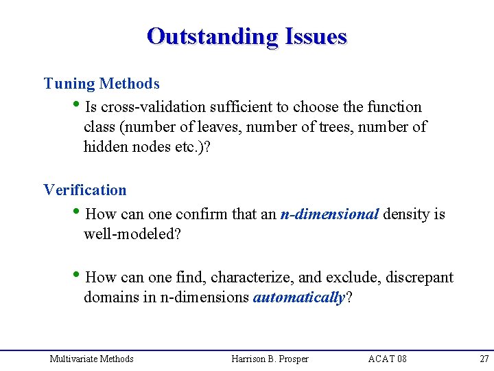
Outstanding Issues Tuning Methods h. Is cross-validation sufficient to choose the function class (number of leaves, number of trees, number of hidden nodes etc. )? Verification h. How can one confirm that an n-dimensional density is well-modeled? h. How can one find, characterize, and exclude, discrepant domains in n-dimensions automatically? Multivariate Methods Harrison B. Prosper ACAT 08 27

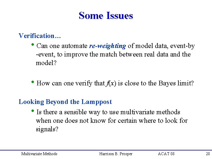
Some Issues Verification… h. Can one automate re-weighting of model data, event-by -event, to improve the match between real data and the model? h. How can one verify that f(x) is close to the Bayes limit? Looking Beyond the Lamppost h. Is there a sensible way to use multivariate methods when one does not know for certain where to look for signals? Multivariate Methods Harrison B. Prosper ACAT 08 28

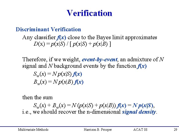
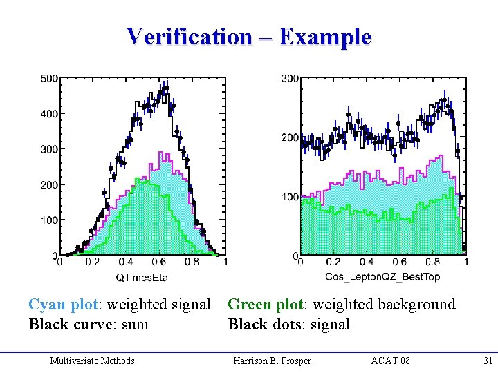
Verification Discriminant Verification Any classifier f(x) close to the Bayes limit approximates D(x) = p(x|S) / [ p(x|S) + p(x|B) ] Therefore, if we weight, event-by-event, an admixture of N signal and N background events by the function f(x) Sw(x) = N p(x|S) f(x) Bw(x) = N p(x|B) f(x) then the sum Sw(x) + Bw(x) = N (p(x|S) + p(x|B)) f(x) = N p(x|S), i. e. , we should recover the n-dimensional signal density. Multivariate Methods Harrison B. Prosper ACAT 08 29

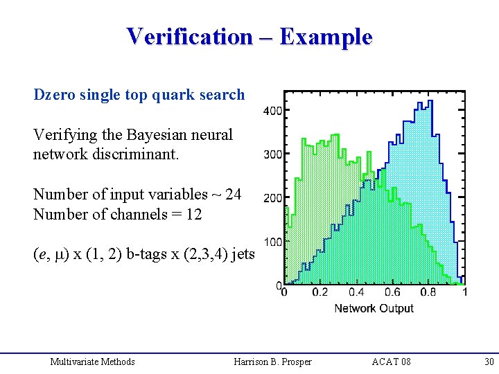
Verification – Example Dzero single top quark search Verifying the Bayesian neural network discriminant. Number of input variables ~ 24 Number of channels = 12 (e, m) x (1, 2) b-tags x (2, 3, 4) jets Multivariate Methods Harrison B. Prosper ACAT 08 30

Verification – Example Cyan plot: weighted signal Green plot: weighted background Black curve: sum Black dots: signal Multivariate Methods Harrison B. Prosper ACAT 08 31

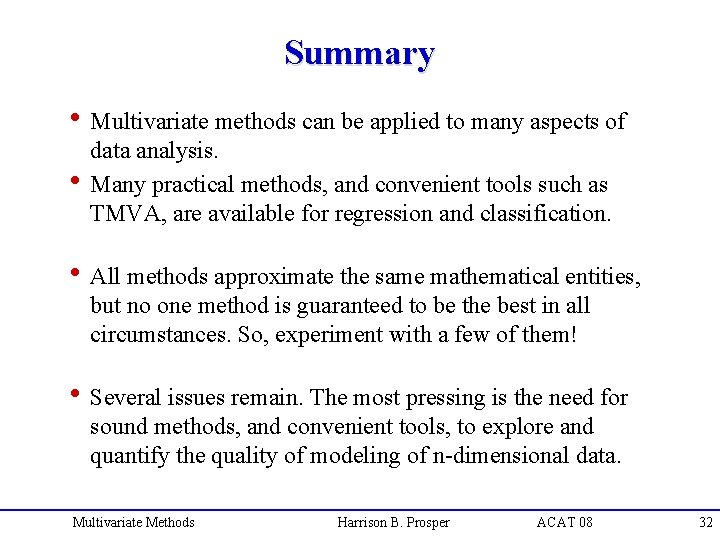
Summary h Multivariate methods can be applied to many aspects of data analysis. h Many practical methods, and convenient tools such as TMVA, are available for regression and classification. h All methods approximate the same mathematical entities, but no one method is guaranteed to be the best in all circumstances. So, experiment with a few of them! h Several issues remain. The most pressing is the need for sound methods, and convenient tools, to explore and quantify the quality of modeling of n-dimensional data. Multivariate Methods Harrison B. Prosper ACAT 08 32