Multiple Imputation with large proportions of missing data

Multiple Imputation with large proportions of missing data : how much is too much? Jin is designed Dr. Huber by Texas A&M HSC

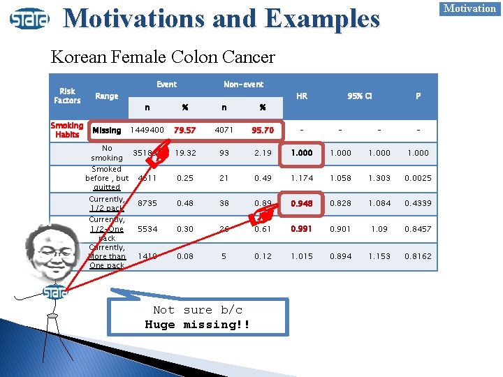
Motivations and Examples Korean Female Colon Cancer Risk Factors Range Smoking Habits Missing Event Non-event HR 95% CI P n % 1449400 79. 57 4071 95. 70 - - 19. 32 93 2. 19 1. 000 0. 25 21 0. 49 1. 174 1. 058 1. 303 0. 0025 0. 48 38 0. 89 0. 948 0. 828 1. 084 0. 4339 0. 30 26 0. 61 0. 991 0. 901 1. 09 0. 8457 0. 08 5 0. 12 1. 015 0. 894 1. 153 0. 8162 No 351896 smoking Smoked before , but 4611 quitted Currently, 8735 1/2 pack Currently, 1/2 -One 5534 pack Currently, More than 1410 One pack ☞ ☞ Not sure b/c Is smoking protective? Huge missing!!

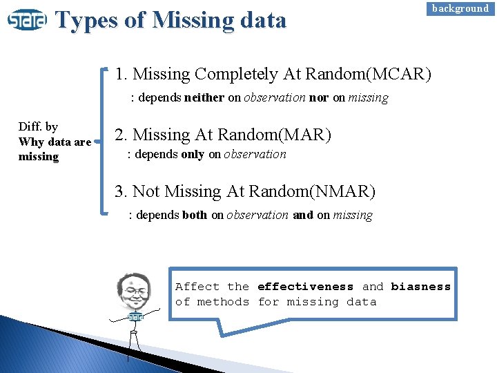
Types of Missing data background 1. Missing Completely At Random(MCAR) : depends neither on observation nor on missing Diff. by Why data are missing 2. Missing At Random(MAR) : depends only on observation 3. Not Missing At Random(NMAR) : depends both on observation and on missing Affect the effectiveness and biasness of methods for missing data

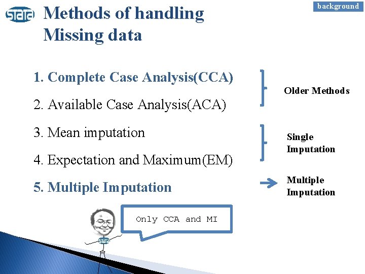
Methods of handling Missing data background 1. Complete Case Analysis(CCA) Older Methods 2. Available Case Analysis(ACA) 3. Mean imputation 4. Expectation and Maximum(EM) 5. Multiple Imputation Only CCA and MI Single Imputation Multiple Imputation

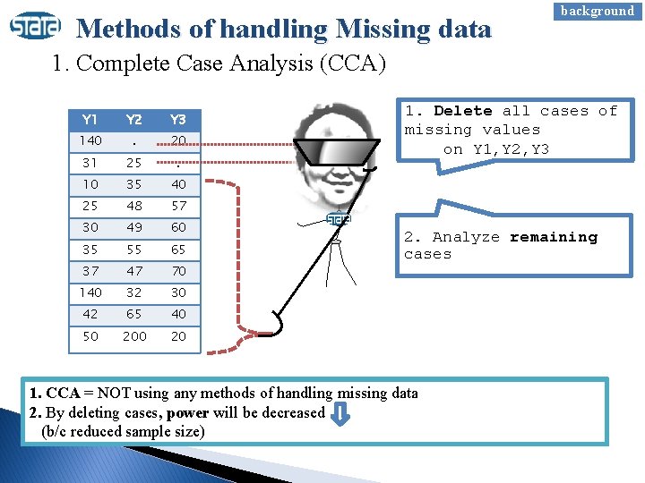
Methods of handling Missing data background 1. Complete Case Analysis (CCA) Y 1 Y 2 Y 3 140 . 20 31 25 . 10 35 40 25 48 57 30 49 60 35 55 65 37 47 70 140 32 30 42 65 40 50 20 1. Delete all cases of missing values on Y 1, Y 2, Y 3 2. Analyze remaining cases 1. CCA = NOT using any methods of handling missing data 2. By deleting cases, power will be decreased (b/c reduced sample size)

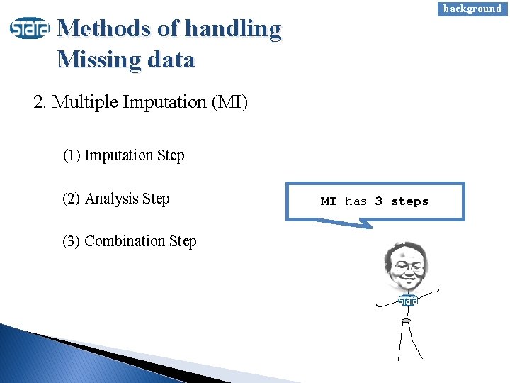
background Methods of handling Missing data 2. Multiple Imputation (MI) (1) Imputation Step (2) Analysis Step (3) Combination Step MI has 3 steps

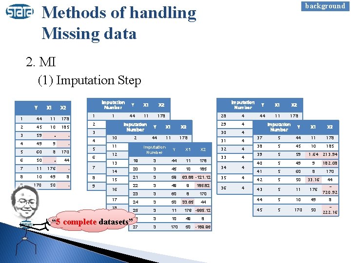
background Methods of handling Missing data 2. MI (1) Imputation Step Y X 1 Imputation Number Y X 1 X 2 1 1 44 11 178 2 1 3 1 10 1 11 1 12 1 13 1 14 1 15 X 2 1 44 11 178 2 45 10 185 3 59 . . 4 49 9 . 5 60 8 170 6 50 . 44 7 11 176 . 7 8 10 49 8 8 9 170 50 . 4 5 6 9 1 16 17 18 45 10 185 Imputation Y X 1 X 2 Number 59 16. 51 136. 48 2 44 11 178 49 9 179. 59 2 45 10 185 Imputation 60 8 170 Y X 1 X 2 Number 2 59 63. 99 -98. 96 50 38. 40 44 19 3 44 11 178 2 49 - 9 192. 37 11 176 20 3608. 57 45 10 185 2 60 8 170 21 49 3 8 59 63. 88 -121. 12 10 2 50 38. 49 44 22 50 3 -88. 94 49 - 9 185. 82 170 2 11 176 23 3 60644. 26 8 170 2 10 49 8 24 3 50 33. 65 44 2 170 50 -97. 00 25 3 11 176 -665. 12 26 “ 5 complete datasets” 27 3 10 49 8 3 170 50 -189. 96 Imputation Number Y X 1 X 2 28 4 44 11 178 29 4 30 4 31 4 32 4 33 4 34 4 35 4 36 4 45 Imputation 10 185 Y Number 59 -42. 87 458. 60 37 5 44 49 9 179. 07 38 5 45 60 8 170 39 5 59 50 33. 60 44 40 5 -49 11 176 41 5 706. 87 60 10 49 8 42 5 50 X 1 X 2 11 178 10 185 1. 64 213. 94 9 182. 08 8 170 33. 16 44 176 720. 92 50 5 11 212. 18 44 5 10 49 8 45 5 170 50 222. 16 170 43

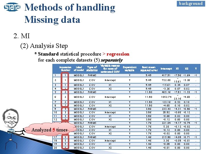
background Methods of handling Missing data 2. MI (2) Analysis Step * Standard statistical procedure > regression for each complete datasets (5) separately Variable names for rows of estimated COV Dependent variable Root mean squared error Intercept Y 9. 49 417. 91 COV Intercept Y 9. 49 MODEL 1 COV PARMS X 1 X 2 Y Y Y 9. 49 11. 80 2 MODEL 1 COV Intercept Y 11. 80 2 2 3 3 4 4 5 5 MODEL 1 MODEL 1 MODEL 1 MODEL 1 COV COV PARMS COV COV X 1 X 2 Y Y Y Y 11. 80 3. 86 1. 76 1. 46 Imputation Number Label of model Type of statistics 1 1 MODEL 1 PARMS 2 1 MODEL 1 3 4 5 1 1 2 6 7 8 9 10 11 12 13 14 15 16 17 18 19 20 Analyzed 5 times Intercept X 1 X 2 X 1 -7. 96 722. 00 15. 61 -15. 61 0. 34 -3. 26 0. 07 405. 16 -7. 81 1052. 74 23. 16 -23. 16 0. 52 -4. 60 0. 10 233. 43 -4. 31 28. 82 -0. 66 0. 02 -0. 12 0. 00 221. 04 -4. 17 5. 20 -0. 12 0. 00 -0. 02 0. 00 215. 80 -4. 08 3. 36 -0. 08 0. 00 -0. 01 0. 00 X 2 Y -1. 64 -1 -3. 26 . 0. 07 0. 02 -1. 53 . . -1 -4. 60 . 0. 10 0. 02 -0. 80 -0. 12 0. 00 -0. 74 -0. 02 0. 00 -0. 71 -0. 01 0. 00 . . -1. . .

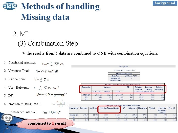
Methods of handling Missing data background 2. MI (3) Combination Step > the results from 5 data are combined to ONE with combination equations. 1. Combined estimate: 2. Variance Total: 3. Var. Within: 4. Var. Between: 5. DF: 6. Fraction missing Info. : 7. Confidence Interval: combined to 1 result

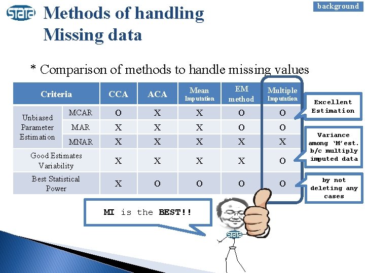
background Methods of handling Missing data * Comparison of methods to handle missing values Multiple Imputation EM method X X O O X X X Good Estimates Variability X X O Best Statistical Power X O O Criteria Unbiased Parameter Estimation CCA ACA MCAR O MAR MNAR Mean MI is the BEST!! Imputation Excellent Estimation Variance among ‘M’est. b/c multiply imputed data by not deleting any cases

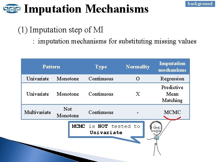
background Imputation Mechanisms (1) Imputation step of MI : imputation mechanisms for substituting missing values Pattern Univariate Monotone Type Normality Imputation mechanisms Continuous O Regression Univariate Monotone Continuous X Predictive Mean Matching Multivariate Not Monotone Continuous - MCMC is NOT tested to Univariate

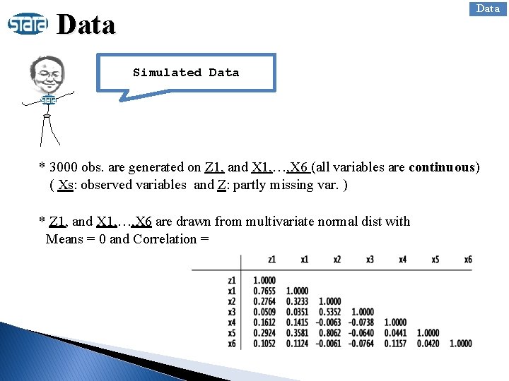
Data Simulated Data * 3000 obs. are generated on Z 1, and X 1, …, X 6 (all variables are continuous) ( Xs: observed variables and Z: partly missing var. ) * Z 1, and X 1, …, X 6 are drawn from multivariate normal dist with Means = 0 and Correlation =

Data Example Data (“A Predictive Study of Coronary Heart Disease” ) * 3154 obs. (all variables are continuous) - Missing variable: Systolic Blood Pressure (Mean: 128. 63) - Observed variables: DBP(82. 02), height(69. 78), weight(169. 95), age(46. 28), BMI(24. 52), and Cholesterol (Mean: 226. 37) * Correlation =

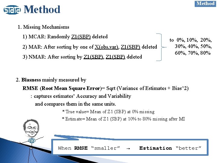
Method 1. Missing Mechanisms 1) MCAR: Randomly Z 1(SBP) deleted 2) MAR: After sorting by one of X(obs. var), Z 1(SBP) deleted 3) NMAR: After sorting by Z 1(SBP), Z 1(SBP) deleted to 0%, 10%, 20%, 30%, 40%, 50%, 60%, 70%, 80% 2. Biasness mainly measured by RMSE (Root Mean Square Error)= Sqrt (Variance of Estimates + Bias^2) : captures estimates’ Accuracy and Variability and compares them in the same units. * True value= Mean of Z 1 (SBP) at 0% missing * Estimate= Mean of Z 1 (SBP) at 10% to 80% missing after MI When RMSE “smaller” → Estimation “better”

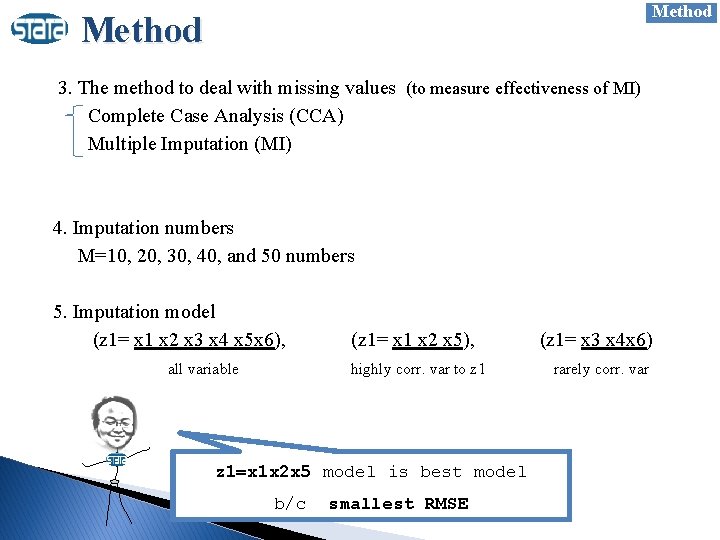
Method 3. The method to deal with missing values (to measure effectiveness of MI) Complete Case Analysis (CCA) Multiple Imputation (MI) 4. Imputation numbers M=10, 20, 30, 40, and 50 numbers 5. Imputation model (z 1= x 1 x 2 x 3 x 4 x 5 x 6), all variable (z 1= x 1 x 2 x 5), highly corr. var to z 1=x 1 x 2 x 5 model is best model b/c smallest RMSE (z 1= x 3 x 4 x 6) rarely corr. var

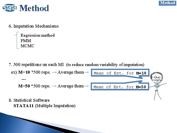
Method 6. Imputation Mechanisms Regression method PMM MCMC 7. 500 repetitions on each MI (to reduce random variability of imputation) ex) M=10 *500 reps. → Average them→ … Mean of Est. for M=10 M=50 *500 reps. → Average them→ Mean of Est. for M=50 8. Statistical Software STATA 11 (Multiple Imputation)

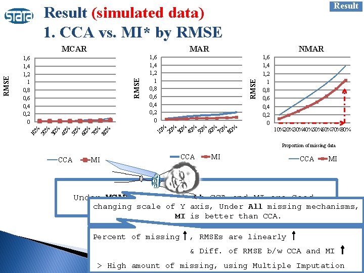
Result (simulated data) 1. CCA vs. MI* by RMSE 1, 6 0, 12 1, 4 0, 1 1, 2 0, 08 1 0, 8 0, 06 0, 04 0, 02 0, 2 00 Proportion of missing data better CCA MI MI 1, 6 0, 25 1, 4 0, 2 1 0, 15 0, 8 0, 6 0, 1 0, 4 0, 05 0, 2 00 NMAR RMSE MAR 1 100% 2% 200% 3% 300% 4% 400% % 5 500% % 6 600% % 7700% % 8800% % RMSE MCAR 0% 0% %0% 0% % % 101 2 303 4 505 6 707 8 Proportion of missing data CCA 1, 6 1, 4 1, 2 1 0, 8 0, 6 0, 4 0, 2 0 10%20%30%40%50%60%70%80% Proportion of missing data MI MI CCA MI Under MCAR and MAR, both CCA and MI are Good. changing scale of Y axis, Under All missing mechanisms, MI is better than CCA. Percent of missing , RMSEs are linearly & Diff. of RMSE b/w CCA and MI > High amount of missing, using Multiple Imputation

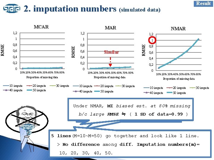
Result 2. imputation numbers (simulated data) MAR NMAR 1, 2 1 1 1 0, 8 0, 6 0, 4 0, 2 0, 6 RMSE 1, 2 RMSE MCAR Similar 0, 4 10%20%30%40%50%60%70%80% Proportion of missing data 10 impute 40 impute 20 impute 50 impute 30 impute 0, 6 0, 4 0, 2 0 0, 8 0, 2 0 10% 20% 30% 40% 50% 60% 70% 80% Proportion of missing data 10 impute 20 impute 40 impute 50 impute 30 impute 0 10%20%30%40%50%60%70%80% Proportion of missing data 10 impute 40 impute 20 impute 50 impute 30 impute Under NMAR, MIof biased est. at (Regardless imputation #)80% missing b/c Under large MCAR RMSE and ≒ (MAR, 1 SDMIof. Good! data=0. 99 ) 5 lines(M=10~M=50) go together and look like 1 line. > No difference among diff. Imputation numbers(m)= 10, 20, 30, 40, 50.

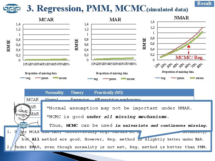
3. Regression, PMM, MCMC(simulated data) MAR 1, 4 1, 2 1 1 1 0, 8 0, 4 1, 2 RMSE 0, 6 0, 4 0, 2 0 0 0 10%20%30%40%50%60%70%80% Proportion of missing data reg pmm Proportion of missing data mcmc NMAR 1, 4 RMSE MCAR reg pmm mcmc MCMC/ Reg. % % % % 10 20 30 40 50 60 70 80 Proportion of missing data reg pmm Normality Theory Practically (MI) MCAR Normal Regression All imputation mechanisms MAR Normal Regression All imputation (Reg. slightly better)NMAR. *Normal assumption may notmechanisms be important under NMAR Not Normal PMM Result mcmc Regression, MCMC *MCMC is good under all missing mechanisms. Thus, MCMC can be used in univariate and continuous missing. 1. Under MCAR and MAR, theoretically Reg. should be better because of normality, but All method are good. However, Reg. method is slightly better under MAR. 2. Under NMAR, even though normality is not met, Reg. method is better than PMM.

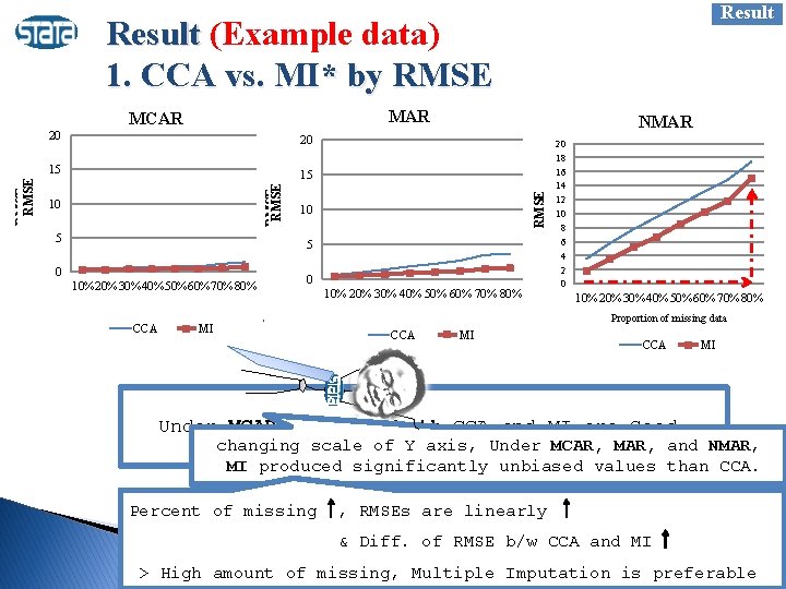
Result (Example data) 1. CCA vs. MI* by RMSE MAR Proportion of missing data CCA MI MI 20 4 3, 5 15 3 2, 5 10 2 1, 5 15 0, 5 00 better NMAR RMSE 20 1, 6 1, 4 15 1, 2 1 10 0, 8 0, 6 5 0, 4 0, 2 0 0 10%20%30%40%50%60%70%80% RMSE MCAR 10%20% 20%30% 30%40% 40%50% 50%60% 60%70% 70%80% 10% Proportion of missing data CCA MI MI 20 18 16 14 12 10 8 6 4 2 0 10% 20% 30% 40% 50% 60% 70% 80% Proportion of missing data CCA MI Under MCAR and MAR, both CCA and MI are Good. changing scale of Y axis, Under MCAR, MAR, and NMAR, MI produced significantly unbiased values than CCA. Percent of missing , RMSEs are linearly & Diff. of RMSE b/w CCA and MI > High amount of missing, Multiple Imputation is preferable

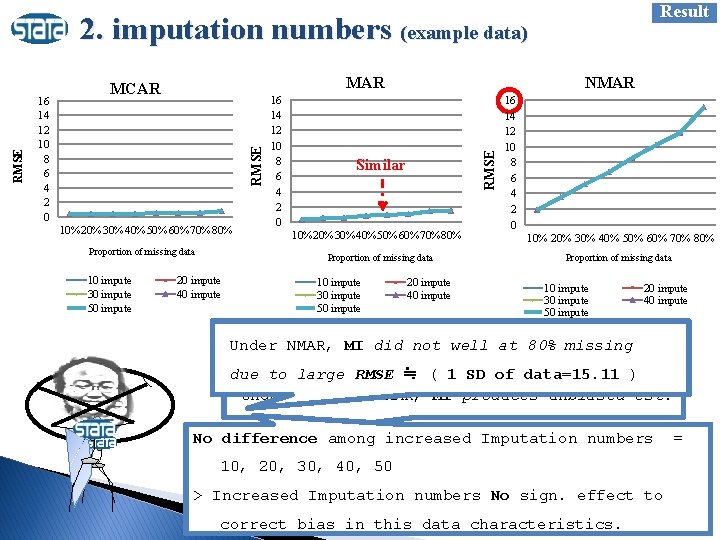
Result 10% 20% 30% 40% 50% 60% 70% 80% Proportion of missing data 10 impute 30 impute 50 impute 16 14 12 10 8 6 4 2 0 NMAR RMSE 16 14 12 10 8 6 4 2 0 MAR MCAR RMSE 2. imputation numbers (example data) Similar 10% 20% 30% 40% 50% 60% 70% 80% Proportion of missing data 20 impute 40 impute 10 impute 30 impute 50 impute 20 impute 40 impute 16 14 12 10 8 6 4 2 0 10% 20% 30% 40% 50% 60% 70% 80% Proportion of missing data 10 impute 30 impute 50 impute 20 impute 40 impute Under NMAR, MI did not well at 80% missing (Regardless of RMSE imputation and of percent of missing due to large ≒ ( 1# SD data=15. 11 ) ) Under MCAR and MAR, MI produces unbiased est. No difference among increased Imputation numbers 10, 20, 30, 40, 50 > Increased Imputation numbers No sign. effect to correct bias in this data characteristics. =

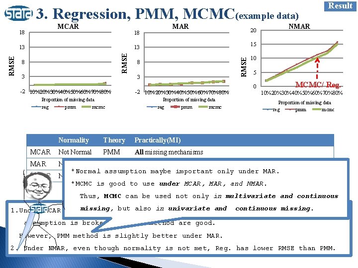
3. Regression, PMM, MCMC(example data) MCAR 18 13 15 3 RMSE 8 8 3 -2 10%20%30%40%50%60%70%80% Proportion of missing data reg pmm -2 10% 20% 30% 40% 50% 60% 70% 80% Proportion of missing data mcmc NMAR 20 13 RMSE MAR 18 reg pmm mcmc 10 5 MCMC/ Reg. 0 10%20%30%40%50%60%70%80% Proportion of missing data reg Normality Theory Practically(MI) MCAR Not Normal PMM All missing mechanisms MAR Not Normal PMM All missing mechanisms (PMM method slightly better ) *Normal assumption maybe important only under MAR. Not Normal PMM Regression, MCMC *MCMC is good to use under MCAR, MAR, and NMAR Result pmm mcmc Thus, MCMC can be used not only in multivariate and continuous but also in PMM univariate andbetter continuous 1. Under MCAR and missing, MAR, theoretically should be becausemissing. normal assumption is broken, but All method are good. However, PMM method is slightly better under MAR. 2. Under NMAR, even though normality is not met, Reg. has lower RMSE than PMM.

Conclusion 1. Multiple Imputation (MI) > Complete Case Analysis always. 2. No significant difference in imputation numbers in my data. 3. Under MCAR and MAR, MI produce unbiased estimates at high amount of missing. 4. However, under NMAR, the estimation by MI is also biased at high amount of missing. 5. MCMC is good for univariate and continuous missing under MCAR, MAR and NMAR.

Thank y u