A Comparison of Approaches to LargeScale Data Analysis

A Comparison of Approaches to Large-Scale Data Analysis Erik Paulson Computer Sciences Department

For later this afternoon Some citations for things I’ll mention today http: //pages. cs. wisc. edu/~epaulson/cs 764 spring 12. html

Today’s Class • Quick Overview of Big Data, Parallel Databases and Map. Reduce • Controversy, or what happens when a blog gets out of hand • A comparison of approaches to large scale data analysis

Lots of data • Google processes 20 PB a day (2008) • Wayback Machine has 3 PB + 100 TB/month (3/2009) • Facebook has 2. 5 PB of user data + 15 TB/day (4/2009) • e. Bay has 6. 5 PB of user data + 50 TB/day (5/2009) • CERN’s LHC will generate 15 PB a year This slide courtesy of Professor Jimmy Lin of UMD, from “Data-Intensive Information Processing Applications” http: //www. umiacs. umd. edu/~jimmylin/cloud-2010 -Spring/

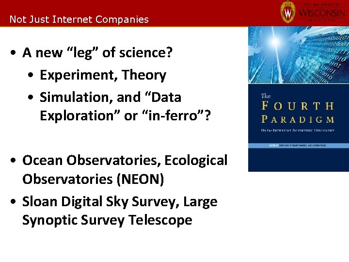
Not Just Internet Companies • A new “leg” of science? • Experiment, Theory • Simulation, and “Data Exploration” or “in-ferro”? • Ocean Observatories, Ecological Observatories (NEON) • Sloan Digital Sky Survey, Large Synoptic Survey Telescope

More Big Data • Netflix and Amazon recommendations • Fraud detection • Google auto-suggest, translation – Also, which ad should you be shown • Full corpus studies in Humanities • Coming soon to campus: early academic intervention

It doesn’t have to be “Big” • Megabytes are still interesting – moving to the web has made integration much easier – Tools are better – Making statistics sexy • More examples – 2012 campaigns – Mashups – Crisis Response – Ushahidi

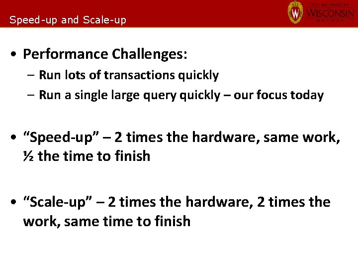
Speed-up and Scale-up • Performance Challenges: – Run lots of transactions quickly – Run a single large query quickly – our focus today • “Speed-up” – 2 times the hardware, same work, ½ the time to finish • “Scale-up” – 2 times the hardware, 2 times the work, same time to finish

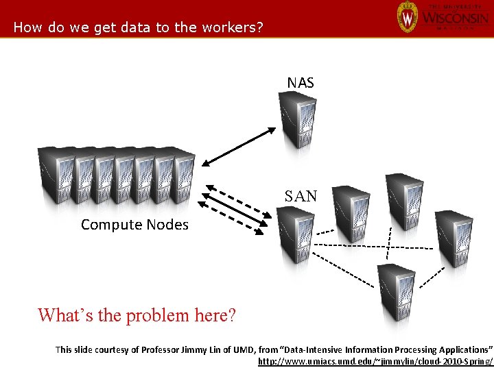
How do we get data to the workers? NAS SAN Compute Nodes What’s the problem here? This slide courtesy of Professor Jimmy Lin of UMD, from “Data-Intensive Information Processing Applications” http: //www. umiacs. umd. edu/~jimmylin/cloud-2010 -Spring/

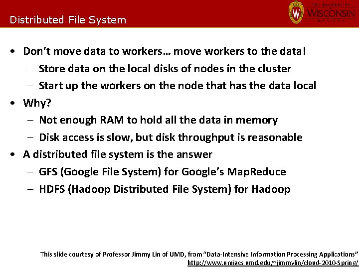
Distributed File System • Don’t move data to workers… move workers to the data! – Store data on the local disks of nodes in the cluster – Start up the workers on the node that has the data local • Why? – Not enough RAM to hold all the data in memory – Disk access is slow, but disk throughput is reasonable • A distributed file system is the answer – GFS (Google File System) for Google’s Map. Reduce – HDFS (Hadoop Distributed File System) for Hadoop This slide courtesy of Professor Jimmy Lin of UMD, from “Data-Intensive Information Processing Applications” http: //www. umiacs. umd. edu/~jimmylin/cloud-2010 -Spring/

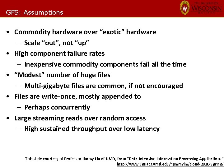
GFS: Assumptions • Commodity hardware over “exotic” hardware – Scale “out”, not “up” • High component failure rates – Inexpensive commodity components fail all the time • “Modest” number of huge files – Multi-gigabyte files are common, if not encouraged • Files are write-once, mostly appended to – Perhaps concurrently • Large streaming reads over random access – High sustained throughput over low latency This slide courtesy of Professor Jimmy Lin of UMD, from “Data-Intensive Information Processing Applications” http: //www. umiacs. umd. edu/~jimmylin/cloud-2010 -Spring/ GFS slides adapted from material by (Ghemawat et al. , SOSP 2003)

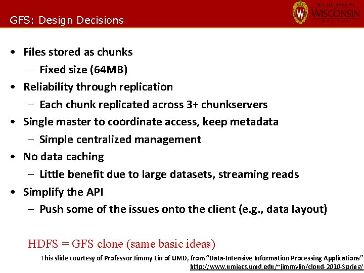
GFS: Design Decisions • Files stored as chunks – Fixed size (64 MB) • Reliability through replication – Each chunk replicated across 3+ chunkservers • Single master to coordinate access, keep metadata – Simple centralized management • No data caching – Little benefit due to large datasets, streaming reads • Simplify the API – Push some of the issues onto the client (e. g. , data layout) HDFS = GFS clone (same basic ideas) This slide courtesy of Professor Jimmy Lin of UMD, from “Data-Intensive Information Processing Applications” http: //www. umiacs. umd. edu/~jimmylin/cloud-2010 -Spring/

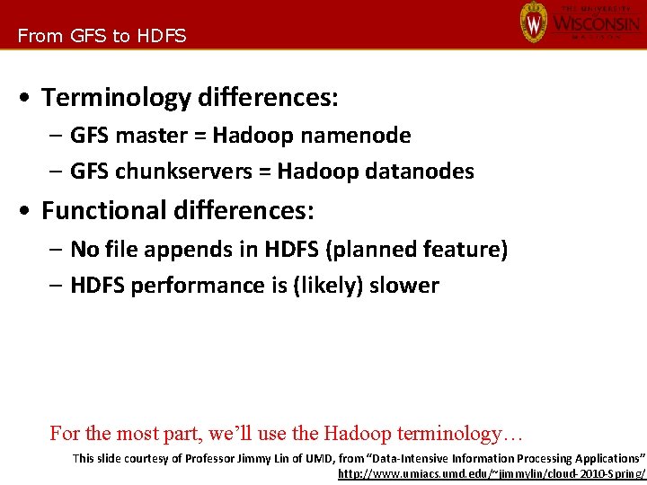
From GFS to HDFS • Terminology differences: – GFS master = Hadoop namenode – GFS chunkservers = Hadoop datanodes • Functional differences: – No file appends in HDFS (planned feature) – HDFS performance is (likely) slower For the most part, we’ll use the Hadoop terminology… This slide courtesy of Professor Jimmy Lin of UMD, from “Data-Intensive Information Processing Applications” http: //www. umiacs. umd. edu/~jimmylin/cloud-2010 -Spring/

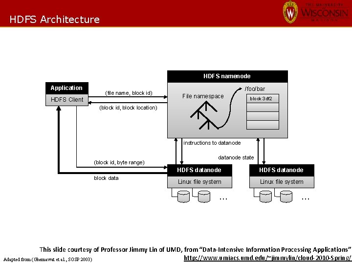
HDFS Architecture HDFS namenode Application (file name, block id) HDFS Client /foo/bar File namespace block 3 df 2 (block id, block location) instructions to datanode (block id, byte range) block datanode state HDFS datanode Linux file system … … This slide courtesy of Professor Jimmy Lin of UMD, from “Data-Intensive Information Processing Applications” http: //www. umiacs. umd. edu/~jimmylin/cloud-2010 -Spring/ Adapted from (Ghemawat et al. , SOSP 2003)

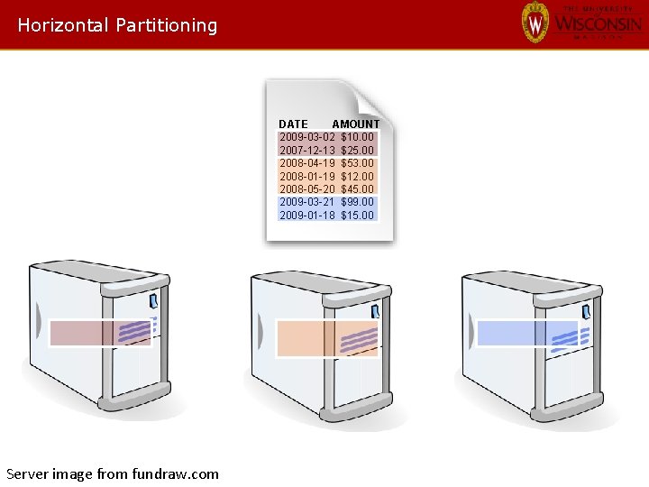
Horizontal Partitioning DATE AMOUNT 2009 -03 -02 $10. 00 2007 -12 -13 $25. 00 2008 -04 -19 $53. 00 2008 -01 -19 $12. 00 2008 -05 -20 $45. 00 2009 -03 -21 $99. 00 2009 -01 -18 $15. 00 Server image from fundraw. com

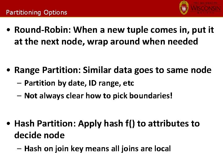
Partitioning Options • Round-Robin: When a new tuple comes in, put it at the next node, wrap around when needed • Range Partition: Similar data goes to same node – Partition by date, ID range, etc – Not always clear how to pick boundaries! • Hash Partition: Apply hash f() to attributes to decide node – Hash on join key means all joins are local

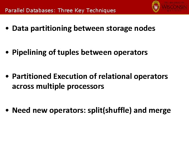
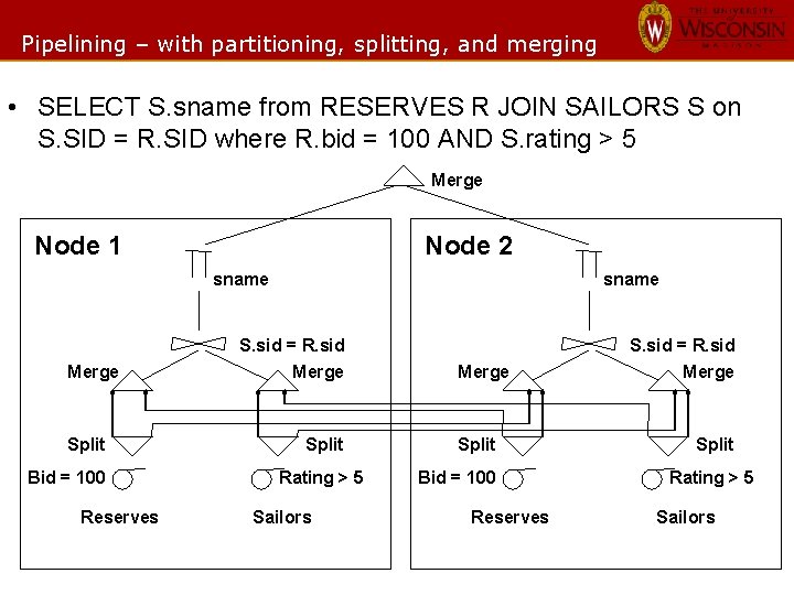
Parallel Databases: Three Key Techniques • Data partitioning between storage nodes • Pipelining of tuples between operators • Partitioned Execution of relational operators across multiple processors • Need new operators: split(shuffle) and merge

Pipelining • SELECT S. sname from RESERVES R JOIN SAILORS S on S. SID = R. SID where R. bid = 100 AND S. rating > 5 Node 1 sname S. sid = R. sid Bid = 100 Reserves Rating > 5 Sailors

Pipelining – with partitioning, splitting, and merging • SELECT S. sname from RESERVES R JOIN SAILORS S on S. SID = R. SID where R. bid = 100 AND S. rating > 5 Merge Node 1 Node 2 sname Merge Split Bid = 100 Reserves sname S. sid = R. sid Merge Split Rating > 5 Sailors Merge Split Bid = 100 Reserves S. sid = R. sid Merge Split Rating > 5 Sailors

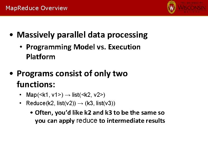
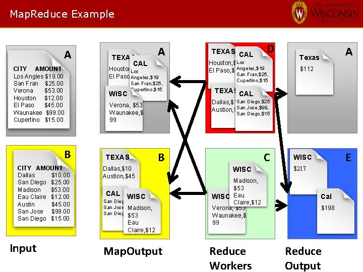
Map. Reduce Overview • Massively parallel data processing • Programming Model vs. Execution Platform • Programs consist of only two functions: • Map(<k 1, v 1>) → list(<k 2, v 2>) • Reduce(k 2, list(v 2)) → (k 3, list(v 3)) • Often, you’d like k 2 and k 3 to be the same so you can apply reduce to intermediate results

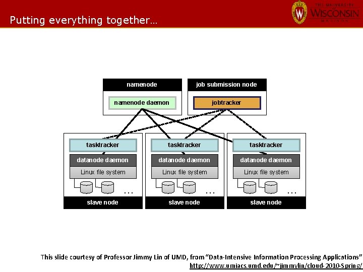
Putting everything together… namenode job submission node namenode daemon jobtracker tasktracker datanode daemon Linux file system … slave node This slide courtesy of Professor Jimmy Lin of UMD, from “Data-Intensive Information Processing Applications” http: //www. umiacs. umd. edu/~jimmylin/cloud-2010 -Spring/

Map. Reduce Example A CITY AMOUNT Los Angles $19. 00 San Fran $25. 00 Verona $53. 00 Houston $12. 00 El Paso $45. 00 Waunakee $99. 00 Cupertino $15. 00 B CITY AMOUNT Dallas $10. 00 San Diego $25. 00 Madison $53. 00 Eau Claire $12. 00 Austin $45. 00 San Jose $99. 00 San Diego $15. 00 Input TEXAS CAL A Houston, $12 Los El Paso, $45 Angeles, $19 San Fran, $25, Cupertino, $15 WISC Los Houston, $12 Angeles, $19 El Paso, $45 San Fran, $25, Cupertino, $15 A Texas $112 TEXAS CAL San Diego, $25 Dallas, $10 San Jose, $99, Austion, $45 Verona, $53 Waunakee, $ 99 TEXAS D TEXAS CAL San Diego, $15 C B Dallas, $10 Austion, $45 CAL WISC San Diego, $25 San Jose, $99, Madison, San Diego, $15 $53 Eau Claire, $12 Map. Output WISC Madison, $53 WISC Eau Claire, $12 Verona, $53 Waunakee, $ 99 Reduce Workers E WISC $217 Cal $198 Reduce Output

The Data Center Is The Computer “I predict Map. Reduce will inspire new ways of thinking about the design and programming of large distributed systems. If Map. Reduce is the first instruction of the ‘data center computer, ’ I can’t wait to see the rest of the instruction set…” -David Patterson Communications of the ACM (January 2008)

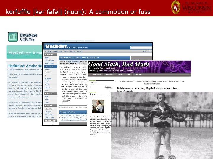
kerfuffle |kərˈfəfəl| (noun): A commotion or fuss

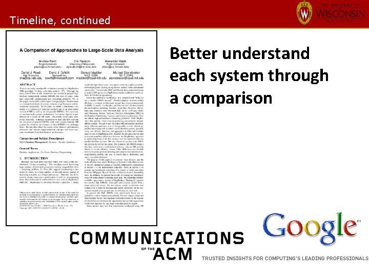
Timeline, continued Map. Reduce or Parallel Database Management Systems (p. DBMS) can be used to analyze large datasets, so appropriate to compare them Proposed a few thought experiments for simple benchmarks

Timeline, continued Better understand each system through a comparison

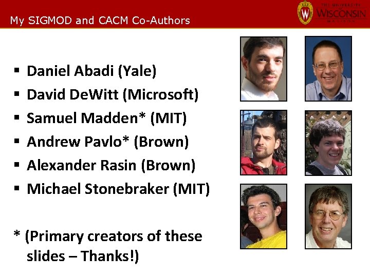
My SIGMOD and CACM Co-Authors § § § Daniel Abadi (Yale) David De. Witt (Microsoft) Samuel Madden* (MIT) Andrew Pavlo* (Brown) Alexander Rasin (Brown) Michael Stonebraker (MIT) * (Primary creators of these slides – Thanks!)

Shared Features • “Shared Nothing” – Cluster fault tolerance – Push plans to local node – Hash or other partitioning for parallelism • Map. Reduce ancestors – Functional programming – Systems community • p. DBMS ancestors – Many 80 s research projects

Differences: Data • Map. Reduce operates on in-situ data, without requiring transformations or loading • Schemas: – Map. Reduce doesn’t require them, DBMSs do – Easy to write simple MR problems – No logical data independence – Google is addressing this with Protocol Buffers, see “Map. Reduce: A Flexible Data Processing Tool” in January 2010 CACM

Differences: Programming Model • Common to write chain of Map. Reduce jobs to perform a task – Analogous to multiple joins/subqueries in DBMSs • No built-in optimizer in Map. Reduce to order or unnest steps • Indexing in Map. Reduce – Possible, but up to the programmer – No optimizer or statistics to select good plan at runtime

Differences: Intermediate Results • Map. Reduce writes intermediate results to disk • p. DBMS usually pushes results to next stage immediately • Map. Reduce trades speed for mid-query fault tolerance – Either system could make other decision – See “Map. Reduce Online” from Berkeley

Map. Reduce and Databases § Understand loading and execution behaviors for common processing tasks. § Large-scale data access (>1 TB): § Analytical query workloads § Bulk loads § Non-transactional § Benchmark § Tasks that either system should execute well

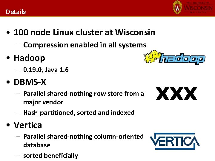
Details • 100 node Linux cluster at Wisconsin – Compression enabled in all systems • Hadoop – 0. 19. 0, Java 1. 6 • DBMS-X – Parallel shared-nothing row store from a major vendor – Hash-partitioned, sorted and indexed • Vertica – Parallel shared-nothing column-oriented database – sorted beneficially XXX

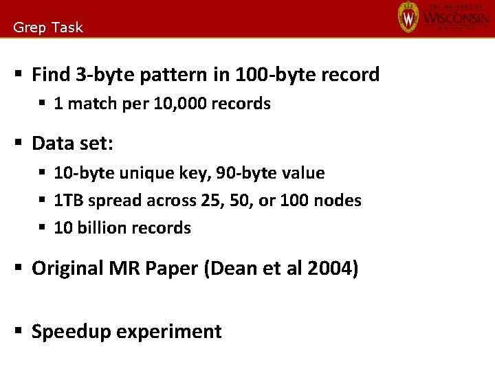
Grep Task § Find 3 -byte pattern in 100 -byte record § 1 match per 10, 000 records § Data set: § 10 -byte unique key, 90 -byte value § 1 TB spread across 25, 50, or 100 nodes § 10 billion records § Original MR Paper (Dean et al 2004) § Speedup experiment

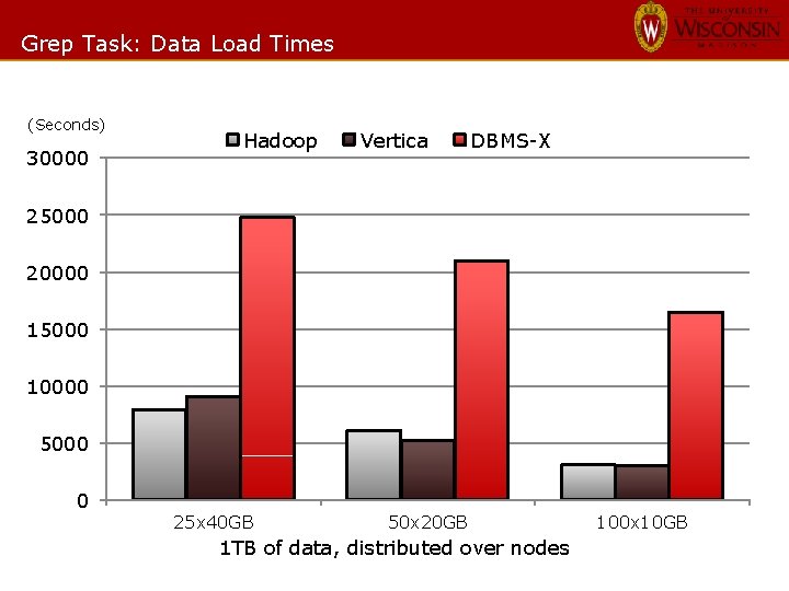
Grep Task: Data Load Times (Seconds) 30000 Hadoop Vertica DBMS-X 25000 20000 15000 10000 5000 0 25 x 40 GB 50 x 20 GB 1 TB of data, distributed over nodes 100 x 10 GB

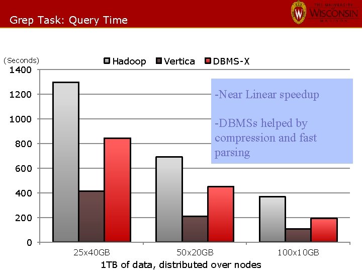
Grep Task: Query Time Hadoop (Seconds) 1400 Vertica DBMS-X 1200 -Near Linear speedup 1000 -DBMSs helped by compression and fast parsing 800 600 400 200 0 25 x 40 GB 50 x 20 GB 1 TB of data, distributed over nodes 100 x 10 GB

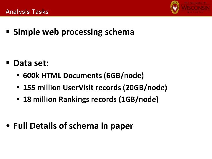
Analysis Tasks § Simple web processing schema § Data set: § 600 k HTML Documents (6 GB/node) § 155 million User. Visit records (20 GB/node) § 18 million Rankings records (1 GB/node) • Full Details of schema in paper

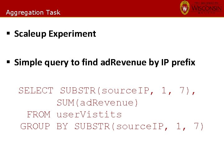
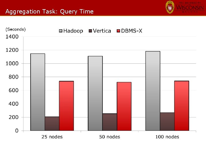
Aggregation Task § Scaleup Experiment § Simple query to find ad. Revenue by IP prefix SELECT SUBSTR(source. IP, 1, 7), SUM(ad. Revenue) FROM user. Vistits GROUP BY SUBSTR(source. IP, 1, 7)

Aggregation Task: Query Time

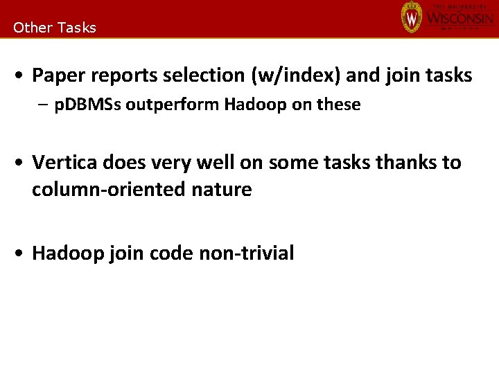
Other Tasks • Paper reports selection (w/index) and join tasks – p. DBMSs outperform Hadoop on these • Vertica does very well on some tasks thanks to column-oriented nature • Hadoop join code non-trivial

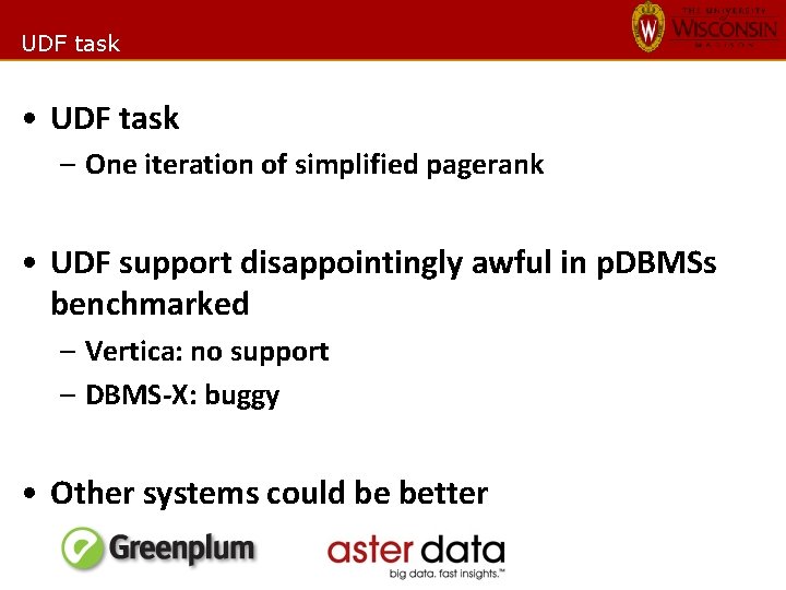
UDF task • UDF task – One iteration of simplified pagerank • UDF support disappointingly awful in p. DBMSs benchmarked – Vertica: no support – DBMS-X: buggy • Other systems could be better

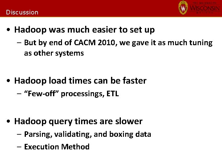
Discussion • Hadoop was much easier to set up – But by end of CACM 2010, we gave it as much tuning as other systems • Hadoop load times can be faster – “Few-off” processings, ETL • Hadoop query times are slower – Parsing, validating, and boxing data – Execution Method

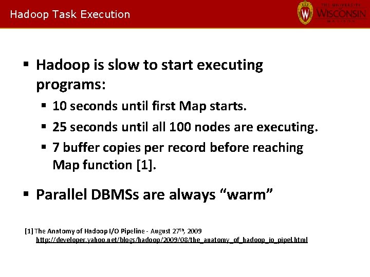
Hadoop Task Execution § Hadoop is slow to start executing programs: § 10 seconds until first Map starts. § 25 seconds until all 100 nodes are executing. § 7 buffer copies per record before reaching Map function [1]. § Parallel DBMSs are always “warm” [1] The Anatomy of Hadoop I/O Pipeline - August 27 th, 2009 http: //developer. yahoo. net/blogs/hadoop/2009/08/the_anatomy_of_hadoop_io_pipel. html

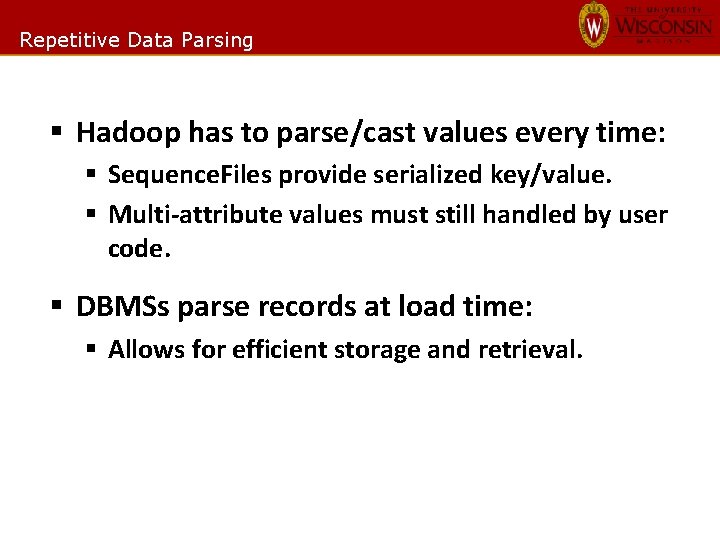
Repetitive Data Parsing § Hadoop has to parse/cast values every time: § Sequence. Files provide serialized key/value. § Multi-attribute values must still handled by user code. § DBMSs parse records at load time: § Allows for efficient storage and retrieval.

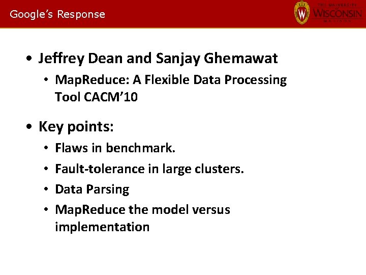
Google’s Response • Jeffrey Dean and Sanjay Ghemawat • Map. Reduce: A Flexible Data Processing Tool CACM’ 10 • Key points: • • Flaws in benchmark. Fault-tolerance in large clusters. Data Parsing Map. Reduce the model versus implementation

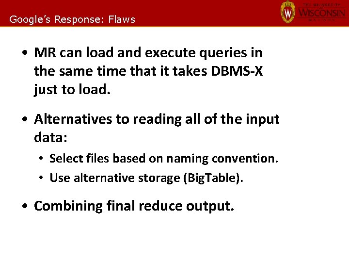
Google’s Response: Flaws • MR can load and execute queries in the same time that it takes DBMS-X just to load. • Alternatives to reading all of the input data: • Select files based on naming convention. • Use alternative storage (Big. Table). • Combining final reduce output.

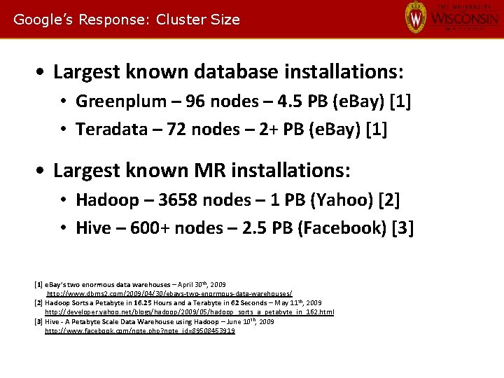
Google’s Response: Cluster Size • Largest known database installations: • Greenplum – 96 nodes – 4. 5 PB (e. Bay) [1] • Teradata – 72 nodes – 2+ PB (e. Bay) [1] • Largest known MR installations: • Hadoop – 3658 nodes – 1 PB (Yahoo) [2] • Hive – 600+ nodes – 2. 5 PB (Facebook) [3] [1] e. Bay’s two enormous data warehouses – April 30 th, 2009 http: //www. dbms 2. com/2009/04/30/ebays-two-enormous-data-warehouses/ [2] Hadoop Sorts a Petabyte in 16. 25 Hours and a Terabyte in 62 Seconds – May 11 th, 2009 http: //developer. yahoo. net/blogs/hadoop/2009/05/hadoop_sorts_a_petabyte_in_162. html [3] Hive - A Petabyte Scale Data Warehouse using Hadoop – June 10 th, 2009 http: //www. facebook. com/note. php? note_id=89508453919

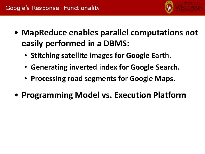
Google’s Response: Functionality • Map. Reduce enables parallel computations not easily performed in a DBMS: • Stitching satellite images for Google Earth. • Generating inverted index for Google Search. • Processing road segments for Google Maps. • Programming Model vs. Execution Platform

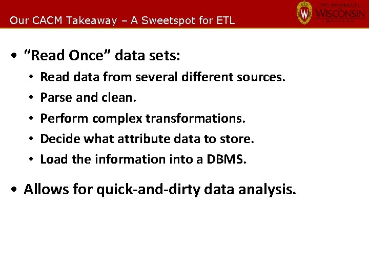
Our CACM Takeaway – A Sweetspot for ETL • “Read Once” data sets: • • • Read data from several different sources. Parse and clean. Perform complex transformations. Decide what attribute data to store. Load the information into a DBMS. • Allows for quick-and-dirty data analysis.

Big Data in the Cloud Age • For about minimum wage, you can have a 100 node cluster – Preconfigured to run Hadoop jobs, no less! • People will use what’s available – The cheaper the better The database community did (does) not have a cheap and ready to download answer for this environment

Take away • Map. Reduce goodness: – Ease of use, immediate results – Attractive fault tolerance – Applicability to other domains – Fast Load Times and in-situ data • Database goodness: – Fast query times – Schemas, indexing, transactions, declarative languages – Supporting tools and enterprise features

Where are we today • Hadoop improvements: – YARN: More flexible execution environment – Better data encoding options: ORCFile, Parquet – Hive and Impala run hot – System catalogs and query optimizers • DBMS Improvements: – More expressive, syntax to run Map. Reduce – External Tables on Distributed Filesystems – Multi Cluster aware/Query planners may run Map. Reduce jobs

Pipelining • SELECT S. sname from RESERVES R JOIN SAILORS S on S. SID = R. SID where R. bid = 100 AND S. rating > 5 Node 1 sname S. sid = R. sid Bid = 100 Reserves Rating > 5 Sailors

• Extra slides

Pipelining – with partitioning, splitting, and merging • SELECT S. sname from RESERVES R JOIN SAILORS S on S. SID = R. SID where R. bid = 100 AND S. rating > 5 Merge Node 1 Node 2 sname Merge Split Bid = 100 Reserves sname S. sid = R. sid Merge Split Rating > 5 Sailors Merge Split Bid = 100 Reserves S. sid = R. sid Merge Split Rating > 5 Sailors

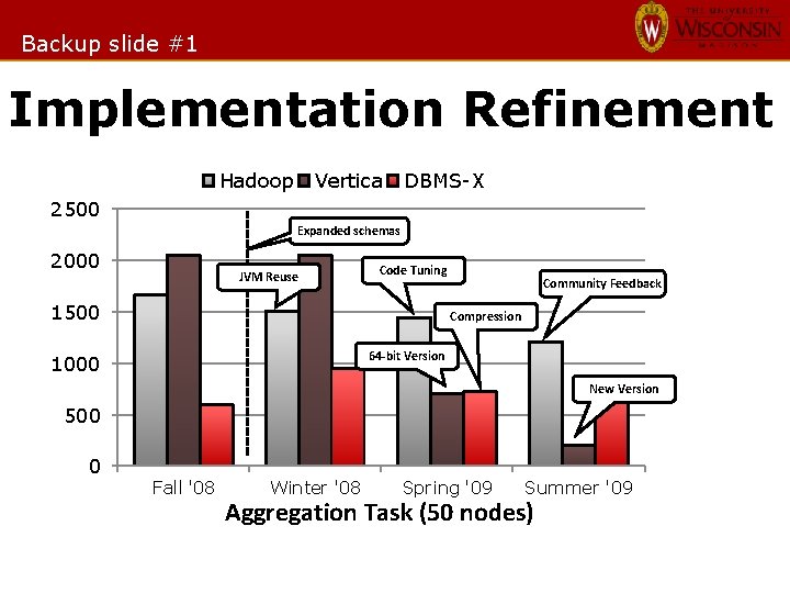
Backup slide #1 Implementation Refinement Hadoop Vertica DBMS-X 2500 Expanded schemas 2000 JVM Reuse Code Tuning 1500 Community Feedback Compression 64 -bit Version 1000 New Version 500 0 Fall '08 Winter '08 Spring '09 Summer '09 Aggregation Task (50 nodes)