Imputation Sarah Medland Boulder 2015 What is imputation

Imputation Sarah Medland Boulder 2015
")
What is imputation? (Marchini & Howie 2010)

• 3 main reasons for imputation • Meta-analysis • Fine Mapping • Combining data from different chips • Other less common uses • sporadic missing data imputation • correction of genotyping errors • imputation of non-SNP variation

Combining data from different chips • Example • 750 individuals typed on the 370 K • 550 individuals typed on the 610 K • Power • MAF. 2 • SNP explaining 1% total variance • alpha 5 e-08 • N=1300, NCP 13. 07, power. 0331 • N=750, NCP 7. 54 , power. 0034 • N=550, NCP 5. 53 , power. 0009

Another way of looking at this

QQ-plot

Solution • Impute all individuals to a single reference based on the SNPs that overlap between the chips • Single distribution of NCP and power across all SNP • qq plot and manhattan describes the full sample with the same degree of accuracy

Ways to approach imputation 1000 Genomes Phase II haplotypes Imputed GWAS genotypes

Imputation programs • minimac 3 • Impute 2 • Beagle – not frequently used • never use plink for imputation!

How do they compare • Similar accuracy • Similar features • Different data formats • minimac 3 –> custom vcf format • individual=row snp=column • Impute 2 –> snp=row individual=column • Different philosophies • Frequentist vs Bayesian

minimac 3 • http: //genome. sph. umich. edu/wiki/Minimac 3 • Built by Gonçalo Abecasis, Yun Li, Christian Fuchsberger and colleagues • Analysis options • raremetalworker (continuous phenotypes & family/twin samples) • Format converter • http: //genome. sph. umich. edu/wiki/Dosage. Convertor • Mach 2 qtl (continuous phenotypes) • Mach 2 dat (binary phenotypes)

Impute 2 • https: //mathgen. stats. ox. ac. uk/impute_v 2. html • http: //genome. sph. umich. edu/wiki/IMPUTE 2: _1000_Genomes_Imputation _Cookbook • Built by Jonathan Marchini, Bryan Howie and colleges • Downstream analysis options • SNPtest • Quicktest

Files to practice with http: //genome. sph. umich. edu/wiki/Minimac 3_Imputation_Cookbook

Today – discuss the 2 step approach Step 1 1000 Genomes Phase II haplotypes Step 2 Imputed GWAS genotypes

Options for imputation • DIY – Use a cookbook! http: //genome. sph. umich. edu/wiki/Minimac 3_Imputation_Cookbo ok OR http: //genome. sph. umich. edu/wiki/IMPUTE 2: _1000_Genomes_Im putation_Cookbook • UMich Imputation Server • https: //imputationserver. sph. umich. edu/ • Sanger Imputation Server • https: //imputation. sanger. ac. uk/

UMich imputation Server

Sanger imputation server

Step 0 – Chose your reference • Current Publically Available References • Hap. Map. II (no phased X data officially released) • Hap. Map. III • 1 KGP – phase 1 version v 3 • 1 KGP – phase 3 version v 5 • Future non-public references only available via custom imputation servers • HRC - 64, 976 haplotypes 39, 235, 157 SNPs • CAPPA – African American/Carabbean • All ethnicities vs specific
")
References are in vcf format (more about this format tomorrow)

Not all references are equal!! The Beagle and IMPUTE versions of the references contain variants that do not appear in the publically available 1 KGP data! The 1 KGP references still contain multiple locations with more than 1 variant & Multiple variants in more than one place!

Step 0 – re-QC your data i. Convert to PLINK binary format ii. Exclude snps with excessive missingness (>5%), low MAF (<1%), HWE violations (~P<10 -4), Mendelian errors iii. Drop all strand ambiguous (palindromic) SNPs – ie A/T or C/G snps iv. Update build and alignment (b 37) v. Check strand! vi. Output your data in the expected format for the phasing program you will use Check the naming convention for the program and reference you want to use rs 278405739 OR 22: 395704

Strand, strand • DNA is a double helix • A pairs with T and C pairs with G • There are two strands: ATCTGGTACTCCAT TAGACCATGAGGTA Strand 1 Strand 2
![Strand, strand • What about SNPs? ATCTGGT[A/C]CTCCAT TAGACCA[T/G]GAGGTA Strand 1 Strand 2](http://slidetodoc.com/presentation_image_h/946b1bc6011b7c70b88757039eec2d5b/image-23.jpg "Strand, strand • What about SNPs? ATCTGGT[A/C]CTCCAT TAGACCA[T/G]GAGGTA Strand 1 Strand 2")
Strand, strand • What about SNPs? ATCTGGT[A/C]CTCCAT TAGACCA[T/G]GAGGTA Strand 1 Strand 2
![Strand, strand • What’s the big/annoying problem? ATCTGGT[A/T]CTCCAT TAGACCA[T/A]GAGGTA Strand 1 Strand 2](http://slidetodoc.com/presentation_image_h/946b1bc6011b7c70b88757039eec2d5b/image-24.jpg "Strand, strand • What’s the big/annoying problem? ATCTGGT[A/T]CTCCAT TAGACCA[T/A]GAGGTA Strand 1 Strand 2")
Strand, strand • What’s the big/annoying problem? ATCTGGT[A/T]CTCCAT TAGACCA[T/A]GAGGTA Strand 1 Strand 2

Strand, strand • Two ambiguous SNP types • A/T and G/C • All others are resolved • How to check? • Allele frequencies [know your population] • LD [if you have raw data] • PLINK and METAL can re-orient strand • Remember the ambiguous ones!

Before we move on to talking about phasing QUESTIONS?

What is phasing • In this context it is really Haplotype Estimation • We take genotype data and try to reconstruct the haplotypes • Can use reference data to improve this estimation

Step 1 - Phasing • Input a diploid target sample and a library of reference haplotypes • Selection of conditioning haplotypes. Eagle 2 first identifies a subset of 10, 000 conditioning haplotypes by ranking reference haplotypes according to the number of discrepancies between each reference haplotype and the homozygous genotypes of the target sample.

• Generation of Hap. Hedge data structure. Eagle 2 next generates a Hap. Hedge data structure on the selected conditioning haplotypes. The Hap. Hedge encodes a sequence of haplo- type prefix trees (i. e. , binary trees on haplotype prefixes) rooted at a sequence of starting positions along the chromosome, thus enabling fast lookup of haplotype frequencies
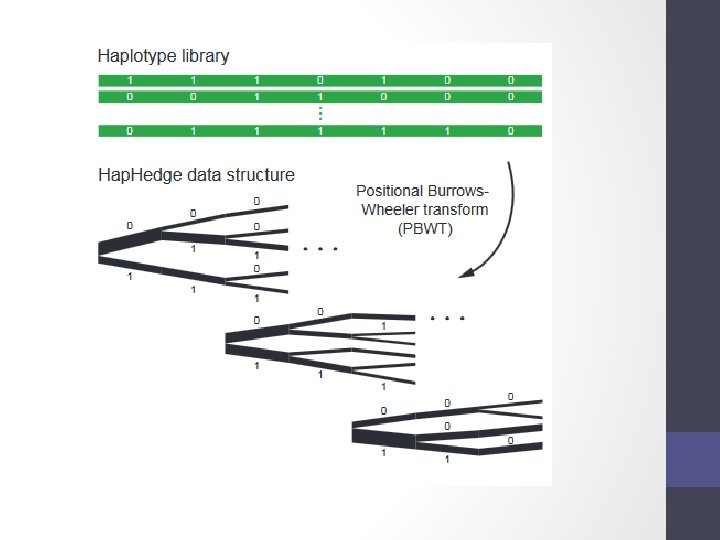

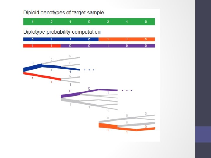
• Exploration of the diplotype space. Having prepared a Hap. Hedge of conditioning haplotypes, Eagle 2 performs phasing using a HMM Consolidates reference haplotypes sharing common prefixes reducing computation.

Step 1 – How to phase Data is usually broken into manageable chunks ~20 Mb Each phased independently. /eagle --vcf. Ref HRC. r 11. GRCh 37. chr 20. shapeit 3. mac 5. aa. genotypes. bcf --vcf. Target chunk_20_000001_0020000000. vcf. gz --genetic. Map. File genetic_map_chr 20_combined_b 37. txt --out. Prefix chunk_20_000001_0020000000. phased --bp. Start 1 --bp. End 25000000 --chrom 20 --allow. Ref. Alt. Swap

Step 2 - Imputation • Compares the phased data to the references and infers the missing genotypes. Calculate accuracy metrics. /Minimac 3 --ref. Haps HRC. r 11. GRCh 37. chr 1. shapeit 3. mac 5. aa. genotypes. m 3 vcf. gz --haps chunk_1_000001_0020000000. phased. vcf --start 1 --end 20000000 --window 500000 --prefix chunk_1_000001_0020000000 --chr 20 --no. Phone. Home --format GT, DS, GP --all. Typed. Sites

Imputing in minimac

Output • Info files

Output • 3 main genotype output formats • Probs format (probability of AA AB and BB genotypes for each SNP) • Hard call or best guess (output as A C T or G allele codes) • Dosage data (most common – 1 number per SNP, 1 -2)

Assessing accuracy of phasing • All phasing methods will make errors in the estimation of haplotypes - probability of error increases with length of imputed region • Problem – some programs are designed to run on small segments others on whole chromosomes • EAGLE 2 currently considered the best • More work needed that compares like with like

Timing & Memory from Das et al 2016 Prior to EAGLE 2

Accuracy of imputation methods

Before we move on to talking about post imputation QC… QUESTIONS?

Post imputation QC • After imputation you need to check that it worked and the data look ok • Things to check • Plot r 2 across each chromosome look to see where it drops off • Plot MAF-reference MAF

Post imputation QC • See meta-analysis section • For each chromosome check N and % of SNPs: • • MAF <. 5% With r 2 0 -. 3, . 3 -. 6, . 6 -1 If you have hard calls or probs data HWE P < 10 E-6 If you have families convert to hard calls and check for Mendelian errors (should be ~. 2%) • % should be roughly constant across chromosomes

Post imputation QC • See meta-analysis session • Next run GWAS for a trait – ideally continuous, calculate lambda and plot: • QQ • Manhattan • SE vs N • P vs Z • Run the same trait on the observed genotypes – plot imputed vs observed

However, if you are running analyses for a consortium they will probably ask you to analyse all variants regardless of whether they pass QC or not… (If you are setting up a meta-analysis consider allowing cohorts to ignore variants with MAF <. 5% and low r 2 – it will save you a lot of time)

2 Issue – the r metrics differ between imputation programs

• In general fairly close correlation • rsq/ Proper. Info/ allelic Rsq • 1 = no uncertainty • 0 = complete uncertainty • . 8 on 1000 individuals = amount of data at the SNP is equivalent to a set of perfectly observed genotype data in a sample size of 800 individuals • Note Mach uses an empirical Rsq (observed var/exp var) and can go above 1

Bad Imputation Better Imputation Good Imputation

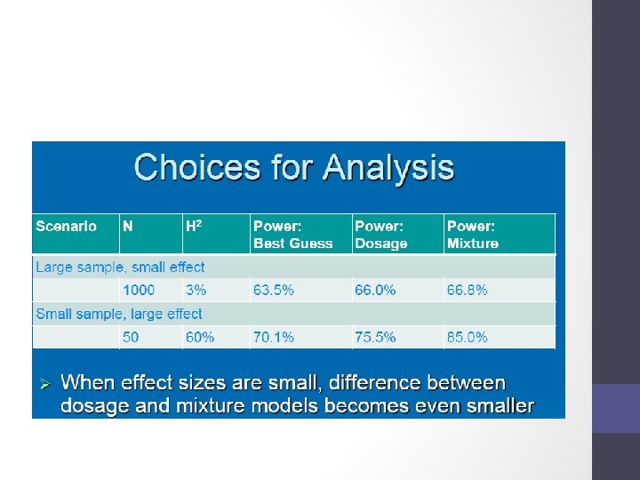
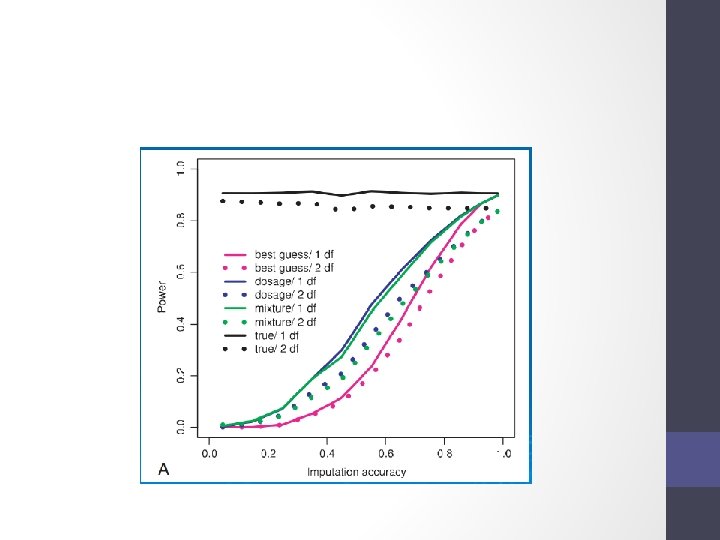
Choices of analysis methods
- Slides: 52