MPE MAP AND APPROXIMATIONS Lecture 10 Statistical Methods

MPE, MAP AND APPROXIMATIONS Lecture 10: Statistical Methods in AI/ML Vibhav Gogate The University of Texas at Dallas Readings: AD Chapter 10

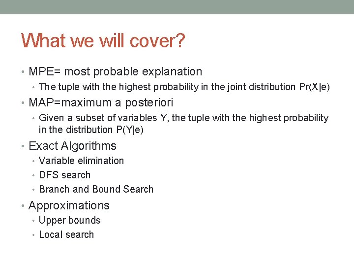
What we will cover? • MPE= most probable explanation • The tuple with the highest probability in the joint distribution Pr(X|e) • MAP=maximum a posteriori • Given a subset of variables Y, the tuple with the highest probability in the distribution P(Y|e) • Exact Algorithms • Variable elimination • DFS search • Branch and Bound Search • Approximations • Upper bounds • Local search

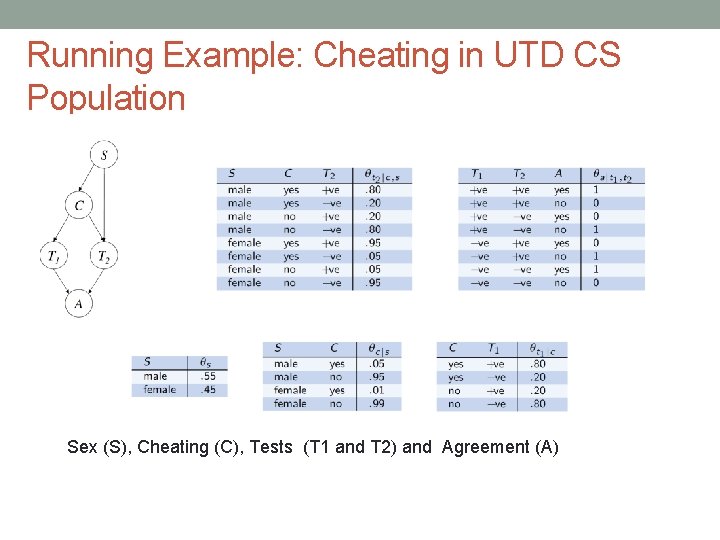
Running Example: Cheating in UTD CS Population Sex (S), Cheating (C), Tests (T 1 and T 2) and Agreement (A)

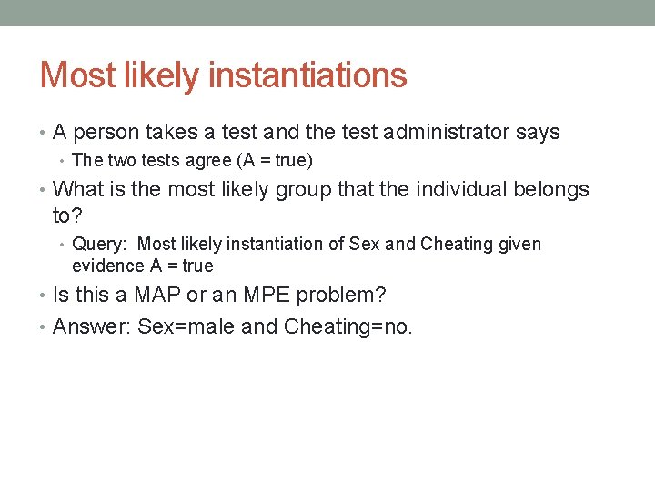
Most likely instantiations • A person takes a test and the test administrator says • The two tests agree (A = true) • What is the most likely group that the individual belongs to? • Query: Most likely instantiation of Sex and Cheating given evidence A = true • Is this a MAP or an MPE problem? • Answer: Sex=male and Cheating=no.

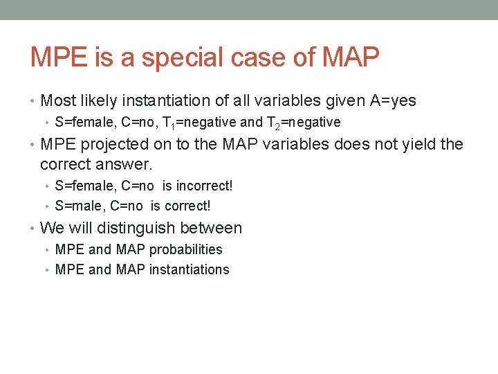
MPE is a special case of MAP • Most likely instantiation of all variables given A=yes • S=female, C=no, T 1=negative and T 2=negative • MPE projected on to the MAP variables does not yield the correct answer. • S=female, C=no is incorrect! • S=male, C=no is correct! • We will distinguish between • MPE and MAP probabilities • MPE and MAP instantiations

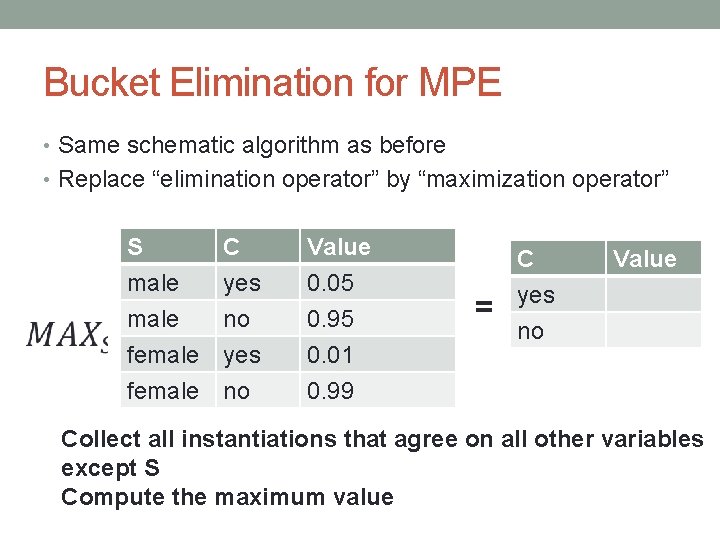
Bucket Elimination for MPE • Same schematic algorithm as before • Replace “elimination operator” by “maximization operator” S male female C yes no yes Value 0. 05 0. 95 0. 01 female no 0. 99 = C yes no Value Collect all instantiations that agree on all other variables except S Compute the maximum value

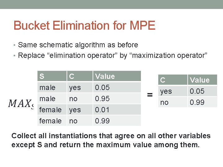
Bucket Elimination for MPE • Same schematic algorithm as before • Replace “elimination operator” by “maximization operator” S male female C yes no yes Value 0. 05 0. 95 0. 01 female no 0. 99 = C yes no Value 0. 05 0. 99 Collect all instantiations that agree on all other variables except S and return the maximum value among them.

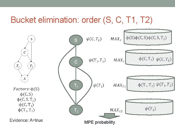
Bucket elimination: order (S, C, T 1, T 2) S C T 1 T 2 MPE probability

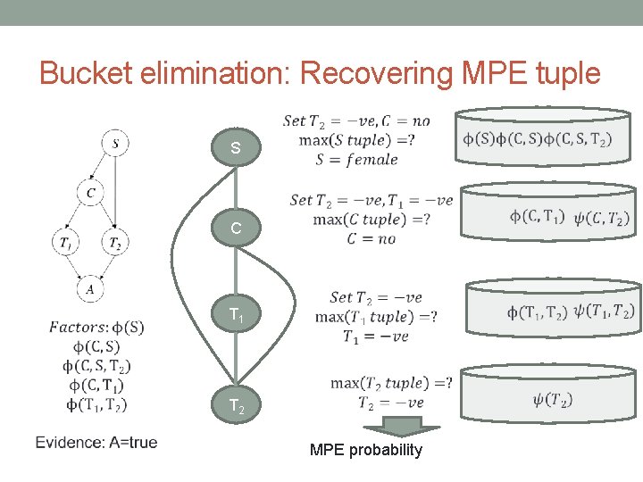
Bucket elimination: Recovering MPE tuple S C T 1 T 2 MPE probability

Bucket elimination: MPE vs PE (Z) • Maximization vs summation • Complexity: Same • Time and Space exponential in the width (w) of the given order: O(n exp(w*+1))

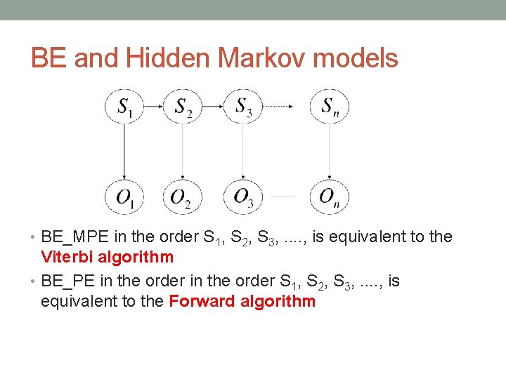
BE and Hidden Markov models • BE_MPE in the order S 1, S 2, S 3, . . , is equivalent to the Viterbi algorithm • BE_PE in the order S 1, S 2, S 3, . . , is equivalent to the Forward algorithm

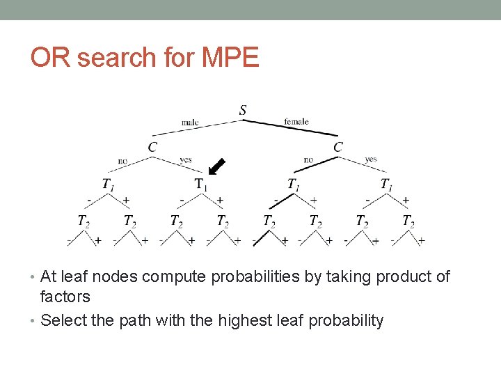
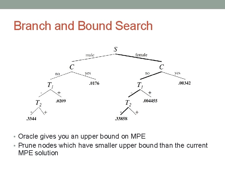
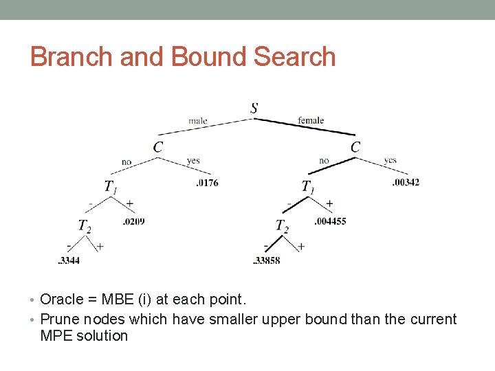
OR search for MPE • At leaf nodes compute probabilities by taking product of factors • Select the path with the highest leaf probability

Branch and Bound Search • Oracle gives you an upper bound on MPE • Prune nodes which have smaller upper bound than the current MPE solution

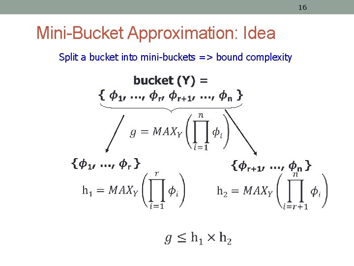
16 Mini-Bucket Approximation: Idea Split a bucket into mini-buckets => bound complexity

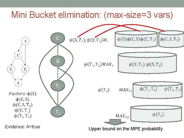
Mini Bucket elimination: (max-size=3 vars) C S T 1 T 2 Upper bound on the MPE probability

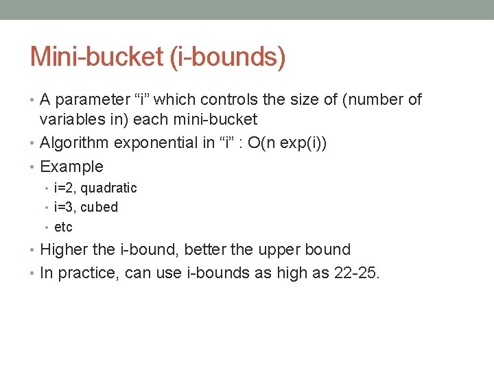
Mini-bucket (i-bounds) • A parameter “i” which controls the size of (number of variables in) each mini-bucket • Algorithm exponential in “i” : O(n exp(i)) • Example • i=2, quadratic • i=3, cubed • etc • Higher the i-bound, better the upper bound • In practice, can use i-bounds as high as 22 -25.

Branch and Bound Search • Oracle = MBE (i) at each point. • Prune nodes which have smaller upper bound than the current MPE solution

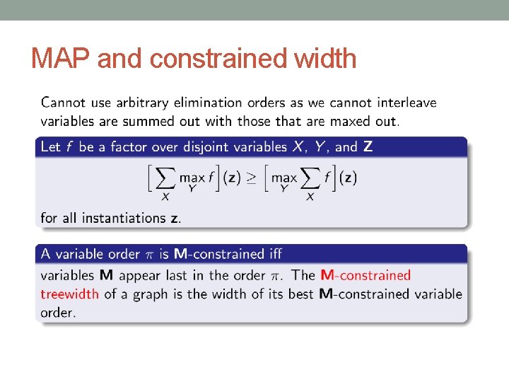
Computing MAP probabilities: Bucket Elimination • Given MAP variables “M” • Can compute the MAP probability using bucket elimination by first summing out all non-MAP variables, and then maximizing out MAP variables. • By summing out non-MAP variables we are effectively computing the joint marginal Pr(M, e) in factored form. • By maximizing out MAP variables M, we are effectively solving an MPE problem over the resulting marginal. • The variable order used in BE_MAP is constrained as it requires MAP variables M to appear last in the order.

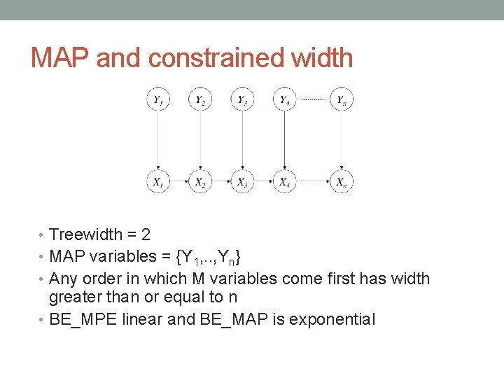
MAP and constrained width • Treewidth = 2 • MAP variables = {Y 1, . . , Yn} • Any order in which M variables come first has width greater than or equal to n • BE_MPE linear and BE_MAP is exponential

MAP and constrained width

MAP by branch and bound search • MAP can be solved using depth-first brand-bound search, just as we did for MPE. • Algorithm BB_MAP resembles the one for computing MPE with two exceptions. • Exception 1: The search space consists only of the MAP variables • Exception 2: We use a version of MBE_MAP for computing the bounds • Order all MAP variables after the non-MAP variables.

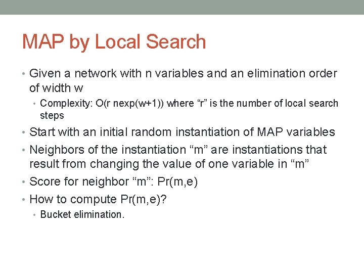
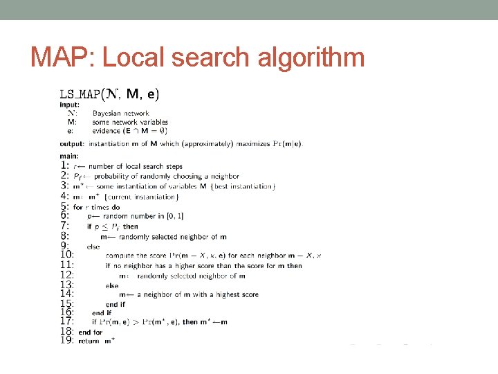
MAP by Local Search • Given a network with n variables and an elimination order of width w • Complexity: O(r nexp(w+1)) where “r” is the number of local search steps • Start with an initial random instantiation of MAP variables • Neighbors of the instantiation “m” are instantiations that result from changing the value of one variable in “m” • Score for neighbor “m”: Pr(m, e) • How to compute Pr(m, e)? • Bucket elimination.

MAP: Local search algorithm

Recap • Exact MPE and MAP • Bucket elimination • Branch and Bound Search • Approximations • Mini bucket elimination • Branch and Bound Search • Local Search