MonteCarlo Tree Search Alan Fern 1 Introduction h

Monte-Carlo Tree Search Alan Fern 1

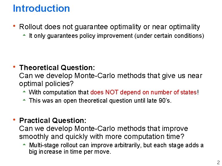
Introduction h Rollout does not guarantee optimality or near optimality 5 It only guarantees policy improvement (under certain conditions) h Theoretical Question: Can we develop Monte-Carlo methods that give us near optimal policies? 5 With computation that does NOT depend on number of states! 5 This was an open theoretical question until late 90’s. h Practical Question: Can we develop Monte-Carlo methods that improve smoothly and quickly with more computation time? 5 Multi-stage rollout can improve arbitrarily, but each stage adds a big increase in time per move. 2

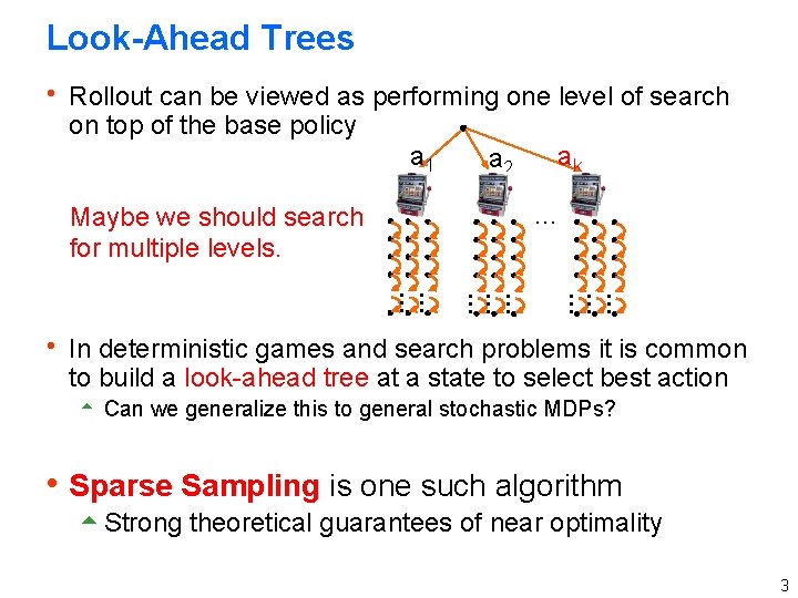
Look-Ahead Trees h Rollout can be viewed as performing one level of search on top of the base policy a 1 a 2 ak … Maybe we should search for multiple levels. … … … … h In deterministic games and search problems it is common to build a look-ahead tree at a state to select best action 5 Can we generalize this to general stochastic MDPs? h Sparse Sampling is one such algorithm 5 Strong theoretical guarantees of near optimality 3

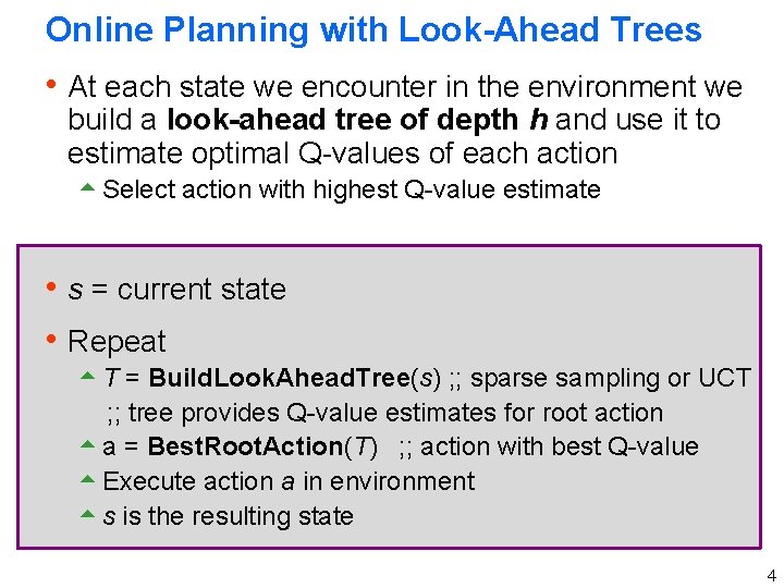
Online Planning with Look-Ahead Trees h At each state we encounter in the environment we build a look-ahead tree of depth h and use it to estimate optimal Q-values of each action 5 Select action with highest Q-value estimate h s = current state h Repeat 5 T = Build. Look. Ahead. Tree(s) ; ; sparse sampling or UCT ; ; tree provides Q-value estimates for root action 5 a = Best. Root. Action(T) ; ; action with best Q-value 5 Execute action a in environment 5 s is the resulting state 4

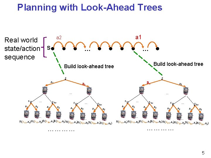
Planning with Look-Ahead Trees a 1 a 2 Real world state/action s sequence … … Build look-ahead tree s s a 1 a 2 … s 11 a 1 … a 2 s 1 w a 1 … s 21 a 2 a 1 … a 2 s 11 s 2 w a 1 a 2 … … R(s 11, a 1) R(s 11, a 2)R(s 1 w, a 1)R(s 1 w, a 2) R(s 21, a 1)R(s , a ) 21 2 2 w 1 2 w 2 ………… a 1 … a 2 s 1 w a 1 s 21 a 2 a 1 … a 2 s 2 w a 1 a 2 … … R(s 11, a 1) R(s 11, a 2)R(s 1 w, a 1)R(s 1 w, a 2) R(s 21, a 1)R(s , a ) 21 2 2 w 1 2 w 2 ………… 5

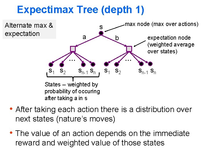
Expectimax Tree (depth 1) Alternate max & expectation max node (max over actions) s a b expectation node (weighted average over states) … … s 1 s 2 sn-1 sn States -- weighted by probability of occuring after taking a in s h After taking each action there is a distribution over next states (nature’s moves) h The value of an action depends on the immediate reward and weighted value of those states

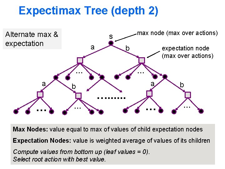
Expectimax Tree (depth 2) Alternate max & expectation max node (max over actions) s a b … a … b … expectation node (max over actions) … a …. . . … b … Max Nodes: value equal to max of values of child expectation nodes Expectation Nodes: value is weighted average of values of its children Compute values from bottom up (leaf values = 0). Select root action with best value.

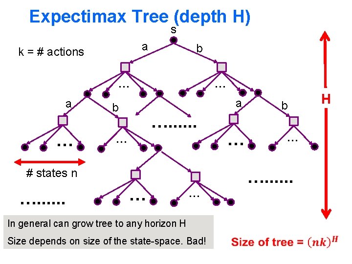
Expectimax Tree (depth H) s a k = # actions b … a …. . . … … # states n … …. . . … … …. . . In general can grow tree to any horizon H Size depends on size of the state-space. Bad! b H

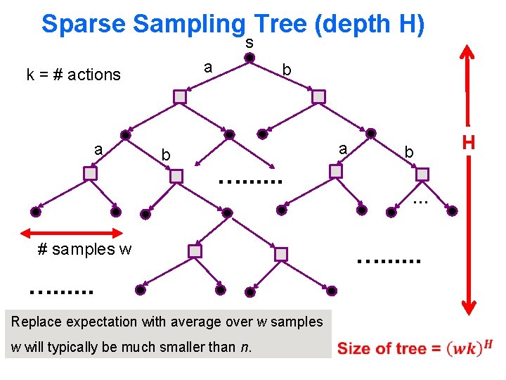
Sparse Sampling Tree (depth H) s a k = # actions a b b a …. . . b … # samples w …. . . Replace expectation with average over w samples w will typically be much smaller than n. H

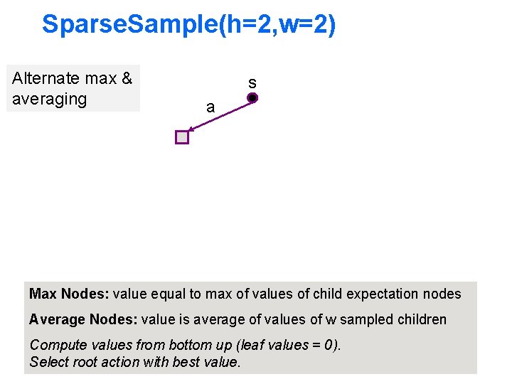
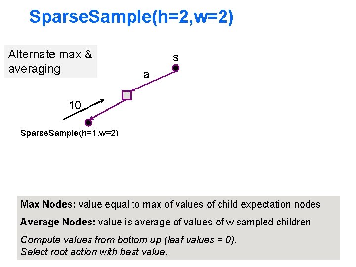
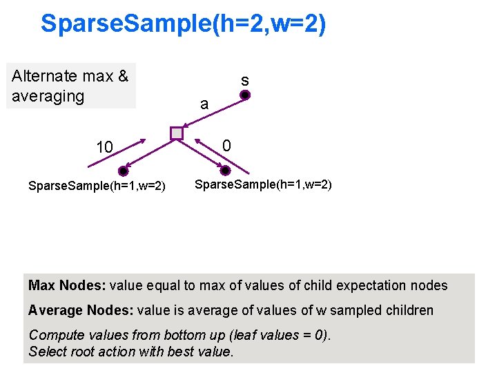
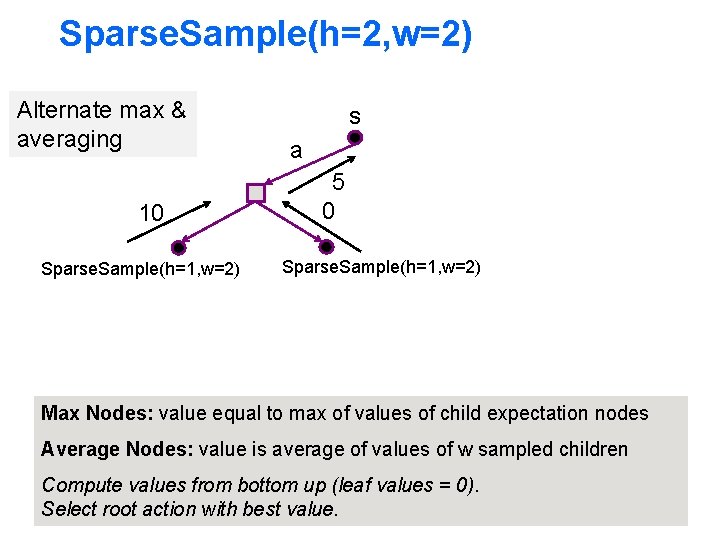
Sparse Sampling [Kearns et. al. 2002] The Sparse Sampling algorithm computes root value via depth first expansion Return value estimate V*(s, h) of state s and estimated optimal action a* Sparse. Sample. Tree(s, h, w) If h == 0 Then Return [0, null] For each action a in s Q*(s, a, h) = 0 For i = 1 to w Simulate taking a in s resulting in si and reward ri [V*(si, h), a*] = Sparse. Sample(si, h-1, w) Q*(s, a, h) = Q*(s, a, h) + ri + β V*(si, h) Q*(s, a, h) = Q*(s, a, h) / w ; ; estimate of Q*(s, a, h) V*(s, h) = maxa Q*(s, a, h) ; ; estimate of V*(s, h) a* = argmaxa Q*(s, a, h) Return [V*(s, h), a*]

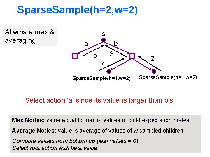
Sparse. Sample(h=2, w=2) Alternate max & averaging s a Max Nodes: value equal to max of values of child expectation nodes Average Nodes: value is average of values of w sampled children Compute values from bottom up (leaf values = 0). Select root action with best value.

Sparse. Sample(h=2, w=2) Alternate max & averaging s a 10 Sparse. Sample(h=1, w=2) Max Nodes: value equal to max of values of child expectation nodes Average Nodes: value is average of values of w sampled children Compute values from bottom up (leaf values = 0). Select root action with best value.

Sparse. Sample(h=2, w=2) Alternate max & averaging 10 Sparse. Sample(h=1, w=2) s a 0 Sparse. Sample(h=1, w=2) Max Nodes: value equal to max of values of child expectation nodes Average Nodes: value is average of values of w sampled children Compute values from bottom up (leaf values = 0). Select root action with best value.

Sparse. Sample(h=2, w=2) Alternate max & averaging 10 Sparse. Sample(h=1, w=2) s a 5 0 Sparse. Sample(h=1, w=2) Max Nodes: value equal to max of values of child expectation nodes Average Nodes: value is average of values of w sampled children Compute values from bottom up (leaf values = 0). Select root action with best value.

Sparse. Sample(h=2, w=2) Alternate max & averaging s b a 3 5 2 4 Sparse. Sample(h=1, w=2) Select action ‘a’ since its value is larger than b’s. Max Nodes: value equal to max of values of child expectation nodes Average Nodes: value is average of values of w sampled children Compute values from bottom up (leaf values = 0). Select root action with best value.

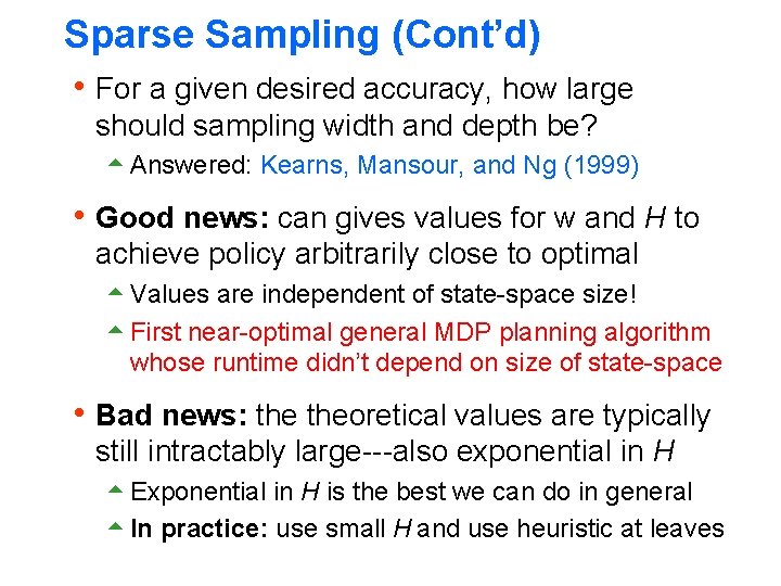
Sparse Sampling (Cont’d) h For a given desired accuracy, how large should sampling width and depth be? 5 Answered: Kearns, Mansour, and Ng (1999) h Good news: can gives values for w and H to achieve policy arbitrarily close to optimal 5 Values are independent of state-space size! 5 First near-optimal general MDP planning algorithm whose runtime didn’t depend on size of state-space h Bad news: theoretical values are typically still intractably large---also exponential in H 5 Exponential in H is the best we can do in general 5 In practice: use small H and use heuristic at leaves

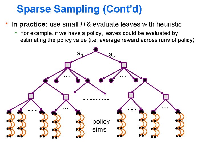
Sparse Sampling (Cont’d) h In practice: use small H & evaluate leaves with heuristic 5 For example, if we have a policy, leaves could be evaluated by estimating the policy value (i. e. average reward across runs of policy) a 1 a 2 … …. . . … policy sims … …

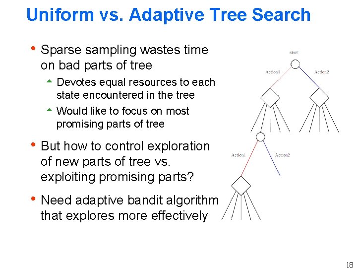
Uniform vs. Adaptive Tree Search h Sparse sampling wastes time on bad parts of tree 5 Devotes equal resources to each state encountered in the tree 5 Would like to focus on most promising parts of tree h But how to control exploration of new parts of tree vs. exploiting promising parts? h Need adaptive bandit algorithm that explores more effectively 18

What now? h Adaptive Monte-Carlo Tree Search 5 UCB Bandit Algorithm 5 UCT Monte-Carlo Tree Search 19

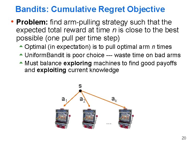
Bandits: Cumulative Regret Objective h Problem: find arm-pulling strategy such that the expected total reward at time n is close to the best possible (one pull per time step) 5 Optimal (in expectation) is to pull optimal arm n times 5 Uniform. Bandit is poor choice --- waste time on bad arms 5 Must balance exploring machines to find good payoffs and exploiting current knowledge s a 1 a 2 ak … 20

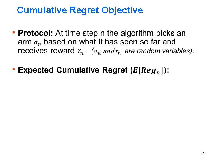
Cumulative Regret Objective 21

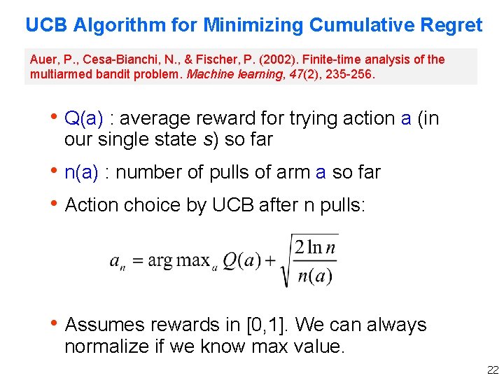
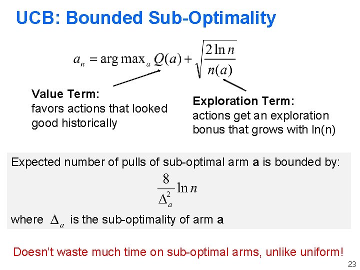
UCB Algorithm for Minimizing Cumulative Regret Auer, P. , Cesa-Bianchi, N. , & Fischer, P. (2002). Finite-time analysis of the multiarmed bandit problem. Machine learning, 47(2), 235 -256. h Q(a) : average reward for trying action a (in our single state s) so far h n(a) : number of pulls of arm a so far h Action choice by UCB after n pulls: h Assumes rewards in [0, 1]. We can always normalize if we know max value. 22

UCB: Bounded Sub-Optimality Value Term: favors actions that looked good historically Exploration Term: actions get an exploration bonus that grows with ln(n) Expected number of pulls of sub-optimal arm a is bounded by: where is the sub-optimality of arm a Doesn’t waste much time on sub-optimal arms, unlike uniform! 23

UCB Performance Guarantee [Auer, Cesa-Bianchi, & Fischer, 2002] h 24

What now? h Adaptive Monte-Carlo Tree Search 5 UCB Bandit Algorithm 5 UCT Monte-Carlo Tree Search 25

UCT Algorithm [Kocsis & Szepesvari, 2006] h UCT is an instance of Monte-Carlo Tree Search 5 Applies principle of UCB 5 Similar theoretical properties to sparse sampling 5 Much better anytime behavior than sparse sampling h Famous for yielding a major advance in computer Go h A growing number of success stories

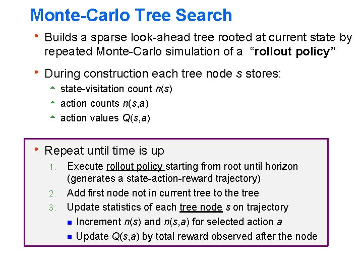
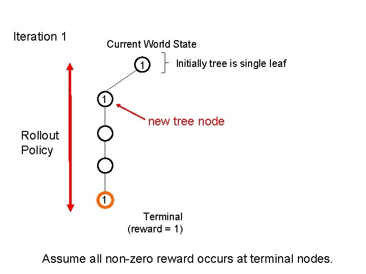
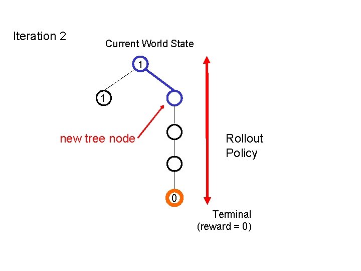
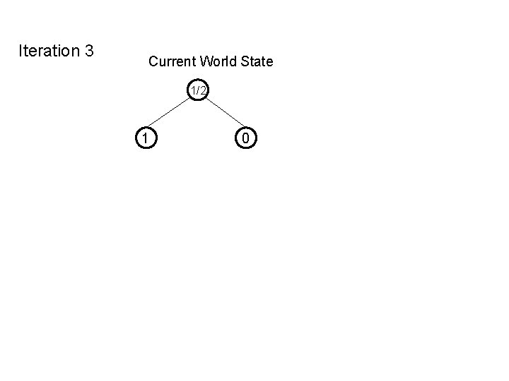
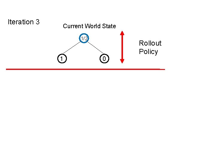
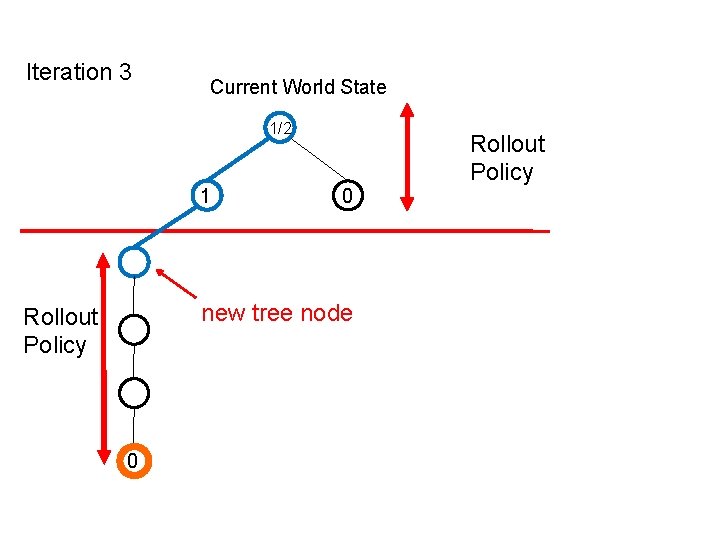
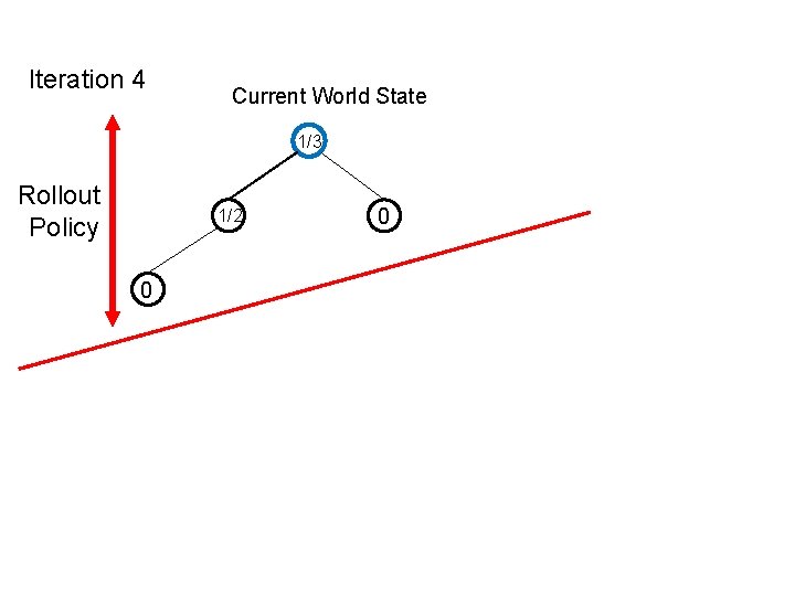
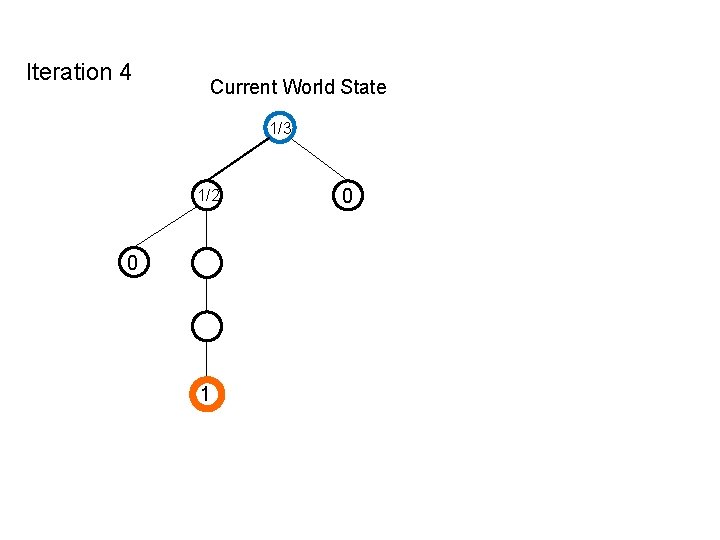
Monte-Carlo Tree Search h Builds a sparse look-ahead tree rooted at current state by repeated Monte-Carlo simulation of a “rollout policy” h During construction each tree node s stores: 5 state-visitation count n(s) 5 action counts n(s, a) 5 action values Q(s, a) h Repeat until time is up 1. Execute rollout policy starting from root until horizon (generates a state-action-reward trajectory) 2. Add first node not in current tree to the tree 3. Update statistics of each tree node s on trajectory g Increment n(s) and n(s, a) for selected action a g Update Q(s, a) by total reward observed after the node

Example MCTS h For illustration purposes we will assume MDP is: 5 Deterministic 5 Only non-zero rewards are at terminal/leaf nodes h Algorithm is well-defined without these assumpitons

Iteration 1 Current World State 1 Initially tree is single leaf 1 new tree node Rollout Policy 1 Terminal (reward = 1) Assume all non-zero reward occurs at terminal nodes.

Iteration 2 Current World State 1 1 new tree node Rollout Policy 0 Terminal (reward = 0)

Iteration 3 Current World State 1/2 1 0

Iteration 3 Current World State 1/2 1 0 Rollout Policy

Iteration 3 Current World State 1/2 1 0 new tree node Rollout Policy 0 Rollout Policy

Iteration 4 Current World State 1/3 Rollout Policy 1/2 0 0

Iteration 4 Current World State 1/3 1/2 0 1 0

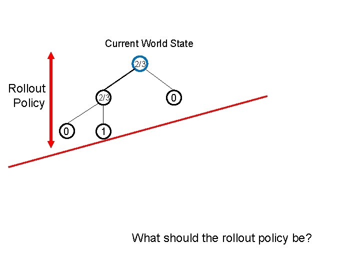
Current World State 2/3 Rollout Policy 2/3 0 0 1 What should the rollout policy be?

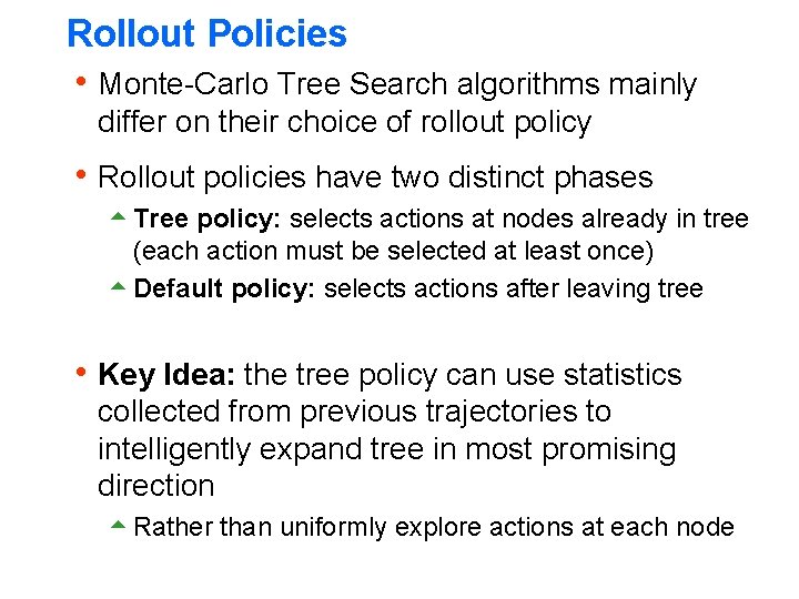
Rollout Policies h Monte-Carlo Tree Search algorithms mainly differ on their choice of rollout policy h Rollout policies have two distinct phases 5 Tree policy: selects actions at nodes already in tree (each action must be selected at least once) 5 Default policy: selects actions after leaving tree h Key Idea: the tree policy can use statistics collected from previous trajectories to intelligently expand tree in most promising direction 5 Rather than uniformly explore actions at each node

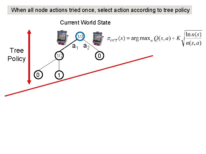
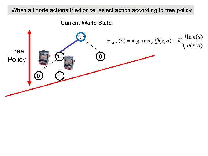
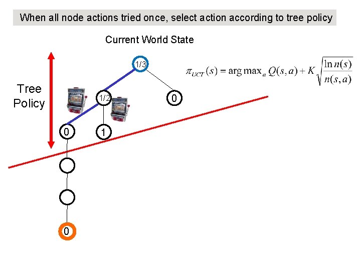
UCT Algorithm [Kocsis & Szepesvari, 2006] h Basic UCT uses random default policy 5 In practice often use hand-coded or learned policy h Tree policy is based on UCB: 5 Q(s, a) : average reward received in trajectories so far after taking action a in state s 5 n(s, a) : number of times action a taken in s 5 n(s) : number of times state s encountered Theoretical constant that must be selected empirically in practice 38

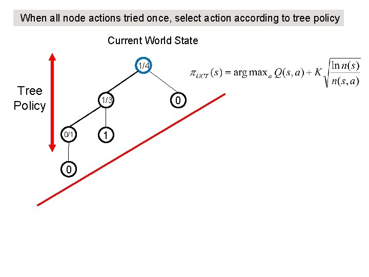
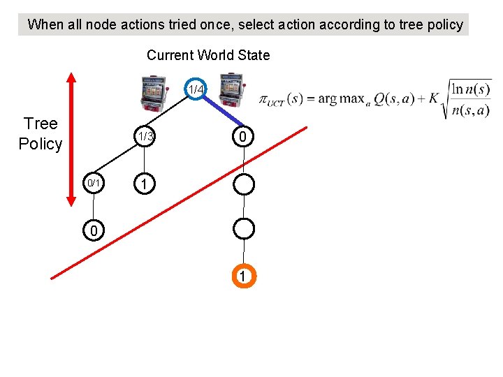
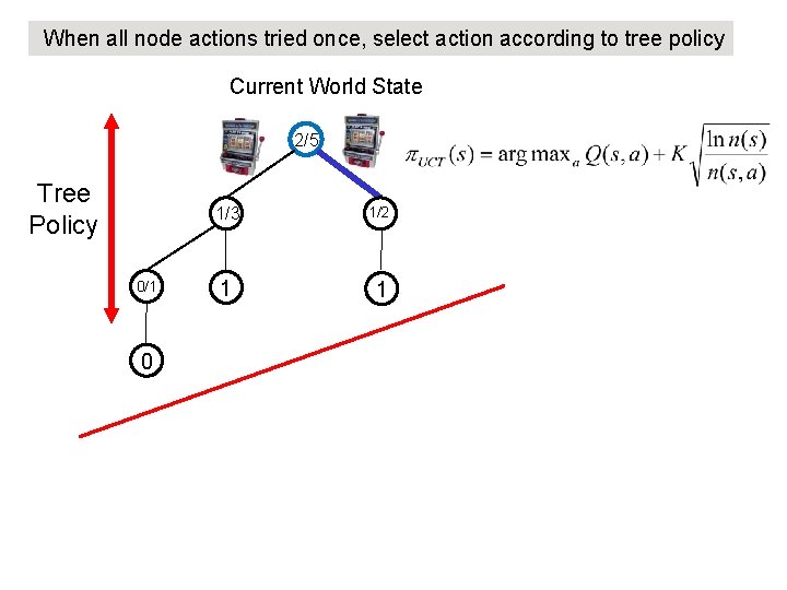
When all node actions tried once, select action according to tree policy Current World State 1/3 a 1 a 2 Tree Policy 1/2 0 1 0

When all node actions tried once, select action according to tree policy Current World State 1/3 Tree Policy 1/2 0 1 0

When all node actions tried once, select action according to tree policy Current World State 1/3 Tree Policy 1/2 0 0 1 0

When all node actions tried once, select action according to tree policy Current World State 1/4 Tree Policy 1/3 0/1 0

When all node actions tried once, select action according to tree policy Current World State 1/4 Tree Policy 1/3 0/1 0 1

When all node actions tried once, select action according to tree policy Current World State 2/5 Tree Policy 0/1 0 1/3 1/2 1 1

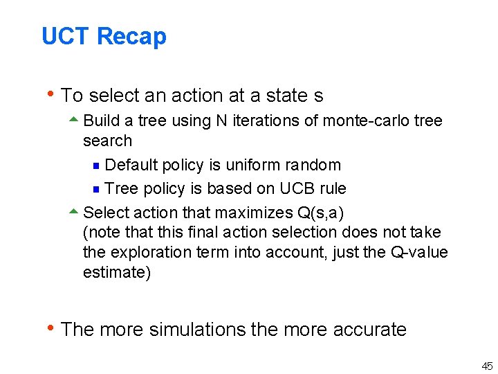
UCT Recap h To select an action at a state s 5 Build a tree using N iterations of monte-carlo tree search g Default policy is uniform random g Tree policy is based on UCB rule 5 Select action that maximizes Q(s, a) (note that this final action selection does not take the exploration term into account, just the Q-value estimate) h The more simulations the more accurate 45

Some Successes Computer Go Klondike Solitaire (wins 40% of games) General Game Playing Competition Real-Time Strategy Games Combinatorial Optimization Crowd Sourcing List is growing Usually extend UCT is some ways

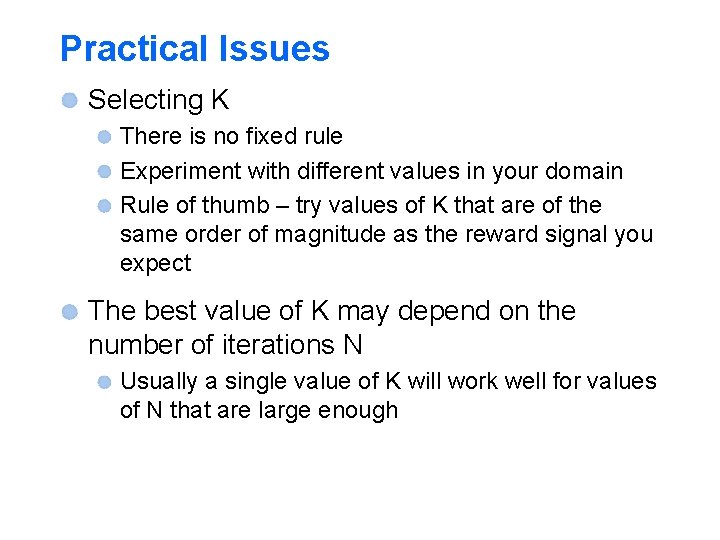
Practical Issues Selecting K There is no fixed rule Experiment with different values in your domain Rule of thumb – try values of K that are of the same order of magnitude as the reward signal you expect The best value of K may depend on the number of iterations N Usually a single value of K will work well for values of N that are large enough

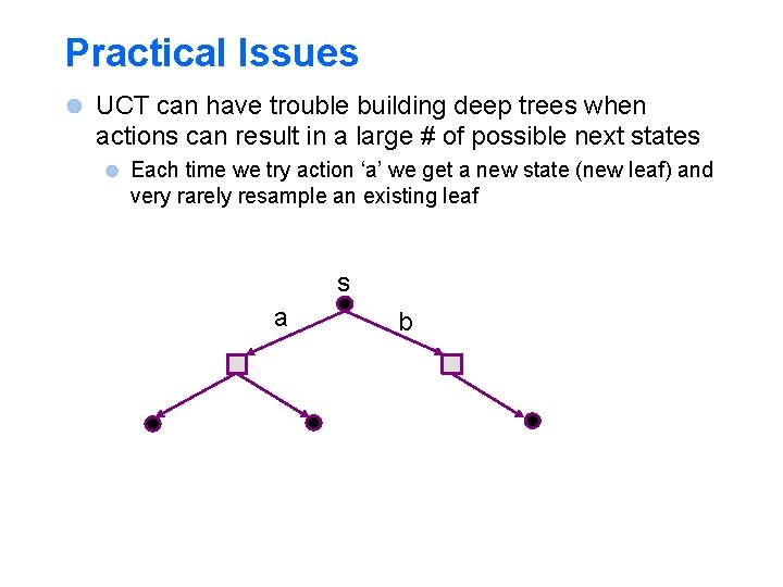
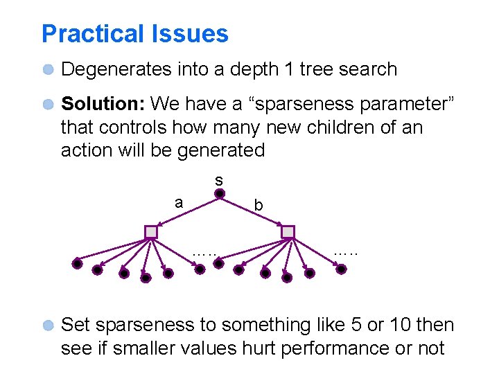
Practical Issues UCT can have trouble building deep trees when actions can result in a large # of possible next states Each time we try action ‘a’ we get a new state (new leaf) and very rarely resample an existing leaf s a b

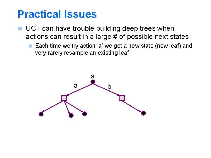
Practical Issues UCT can have trouble building deep trees when actions can result in a large # of possible next states Each time we try action ‘a’ we get a new state (new leaf) and very rarely resample an existing leaf s a b

Practical Issues Degenerates into a depth 1 tree search Solution: We have a “sparseness parameter” that controls how many new children of an action will be generated s a b …. . Set sparseness to something like 5 or 10 then see if smaller values hurt performance or not

Some Improvements Use domain knowledge to handcraft a more intelligent default policy than random E. g. don’t choose obviously stupid actions In Go a hand-coded default policy is used Learn a heuristic function to evaluate positions Use the heuristic function to initialize leaf nodes (otherwise initialized to zero)