MINISTERO DELLINTERNO DIPARTIMENTO DEI VIGILI DEL FUOCO DEL

MINISTERO DELL’INTERNO DIPARTIMENTO DEI VIGILI DEL FUOCO, DEL SOCCORSO PUBBLICO E DELLA DIFESA CIVILE DIREZIONE CENTRALE PER LA FORMAZIONE An Application In Fire Safety Engineering C. Barbera, A. Bascià, G. Di Salvo, A. Galfo, R. Lala, S. Lucidi, D. Maisano, G. Mancini, V. Puccia, F. Vorraro I e II Corso Direttori Antincendi Istituto Superiore Antincendi Roma Fire Service College Moreton-in-Marsh

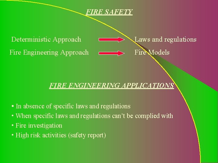
FIRE SAFETY Deterministic Approach Laws and regulations Fire Engineering Approach Fire Models FIRE ENGINEERING APPLICATIONS • In absence of specific laws and regulations • When specific laws and regulations can’t be complied with • Fire investigation • High risk activities (safety report)

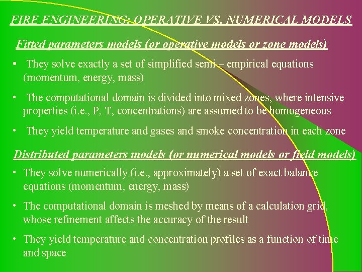
FIRE ENGINEERING: OPERATIVE VS. NUMERICAL MODELS Fitted parameters models (or operative models or zone models) • They solve exactly a set of simplified semi – empirical equations (momentum, energy, mass) • The computational domain is divided into mixed zones, where intensive properties (i. e. , P, T, concentrations) are assumed to be homogeneous • They yield temperature and gases and smoke concentration in each zone Distributed parameters models (or numerical models or field models) • They solve numerically (i. e. , approximately) a set of exact balance equations (momentum, energy, mass) • The computational domain is meshed by means of a calculation grid, whose refinement affects the accuracy of the result • They yield temperature and concentration profiles as a function of time and space

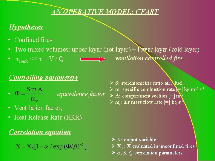
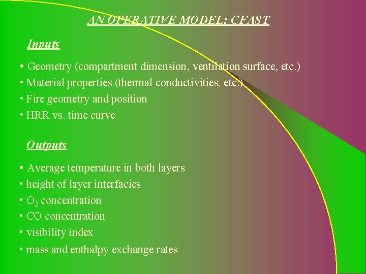
AN OPERATIVE MODEL: CFAST Hypotheses • Confined fires • Two mixed volumes: upper layer (hot layer) + lower layer (cold layer) ventilation controlled fire • tcomb << t = V / Q Controlling parameters • Ø S: stoichiometric ratio air / fuel Ø m: specific combustion rate [=] kg m-2 s-1 equivalence factor Ø A: compartment section [=] m-2 Ø me: air mass flow rate [=] kg s-1 • Ventilation factor, • Heat Release Rate (HRR) Correlation equation Ø X: output variable Ø X 0 : X evaluated in unconfined fires Ø a, b, z: correlation parameters

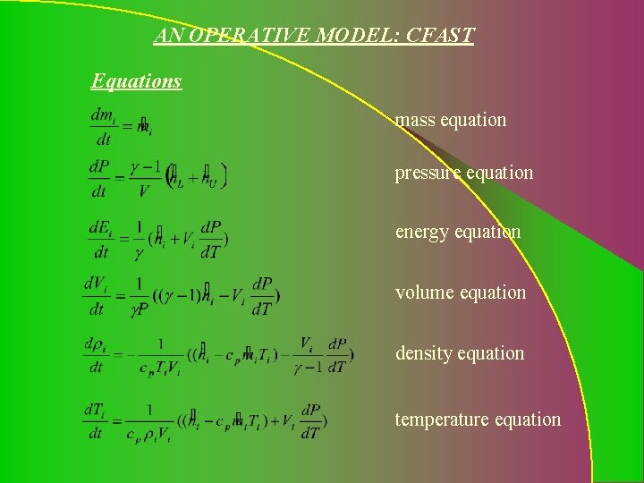
AN OPERATIVE MODEL: CFAST Equations mass equation pressure equation energy equation volume equation density equation temperature equation

AN OPERATIVE MODEL: CFAST Inputs • Geometry (compartment dimension, ventilation surface, etc. ) • Material properties (thermal conductivities, etc. ) • Fire geometry and position • HRR vs. time curve Outputs • Average temperature in both layers • height of layer interfacies • O 2 concentration • CO concentration • visibility index • mass and enthalpy exchange rates

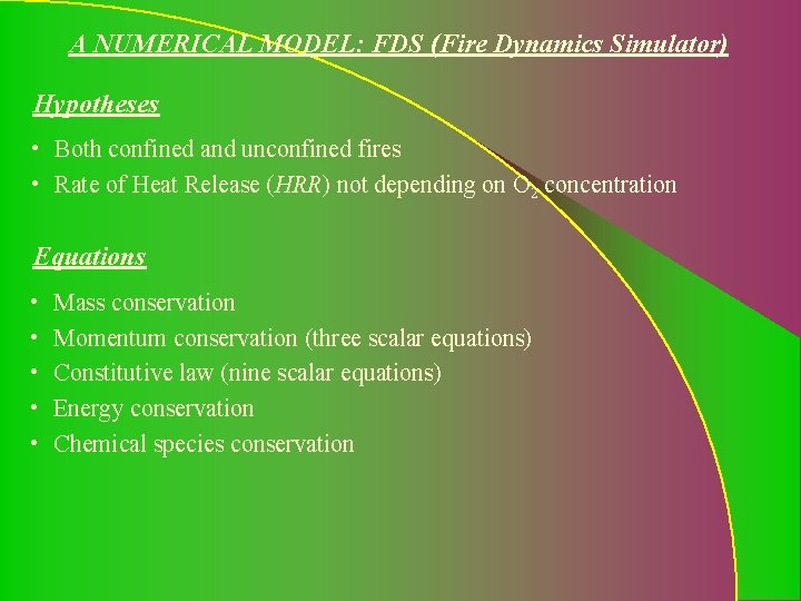
A NUMERICAL MODEL: FDS (Fire Dynamics Simulator) Hypotheses • Both confined and unconfined fires • Rate of Heat Release (HRR) not depending on O 2 concentration Equations • • • Mass conservation Momentum conservation (three scalar equations) Constitutive law (nine scalar equations) Energy conservation Chemical species conservation

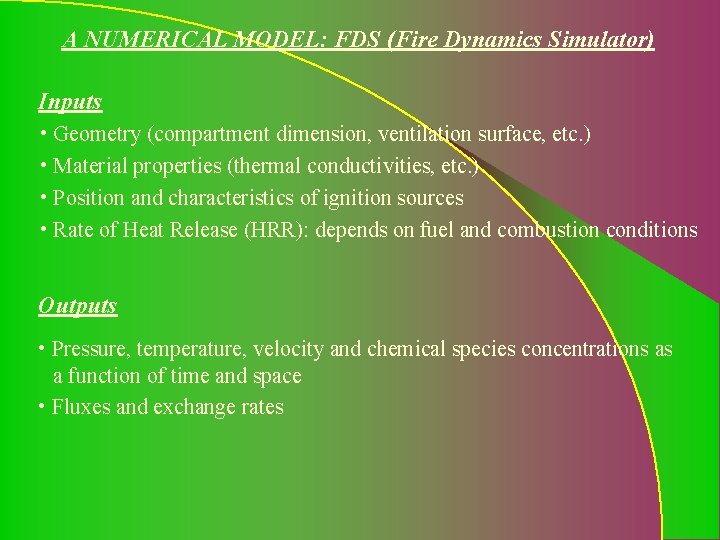
A NUMERICAL MODEL: FDS (Fire Dynamics Simulator) Inputs • Geometry (compartment dimension, ventilation surface, etc. ) • Material properties (thermal conductivities, etc. ) • Position and characteristics of ignition sources • Rate of Heat Release (HRR): depends on fuel and combustion conditions Outputs • Pressure, temperature, velocity and chemical species concentrations as a function of time and space • Fluxes and exchange rates

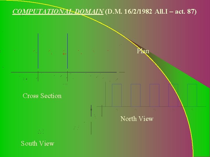
COMPUTATIONAL DOMAIN (D. M. 16/2/1982 All. I – act. 87) Plan Cross Section North View South View

COMPUTATIONAL DOMAIN (D. M. 16/2/1982 All. I – act. 87) • Geometry Two compartments Ventilation surfaces (2 windows + 1 external door + 1 internal door) • Material properties Concrete walls (r = 2100 kg m-3; cp = 0. 88 k. J kg-1 K-1; k. T = 1 W m-1 K-1) • Fire geometry and position 7 cellulosic material stacks • Heat Release Rate (HRR): depends on fuel and combustion conditions

CFAST NUMERICAL RUNS HRR [=] MW t 0 Run 1: sensitivity analysis on the role of a t 1 t 2 t [=] s t 3 Runs a 1 0. 0029 k. W s-2 a 2 0. 0049 k. W s-2 a 3 0. 0069 k. W s-2 a 4 0. 009 k. W s-2 a 5 0. 011 k. W s-2 a 6 0. 02 k. W s-2 HRRmax (MW) 27. 55 32. 83 36. 90 40. 22 42. 97 52. 39 t 0 (s) 0 0 0 t 1 (s) 3080 2585 2300 2110 1975 1620 t 2 (s) 9240 7755 6900 6330 5925 4860 t 3 (s) 12320 10340 9200 8440 7900 6480

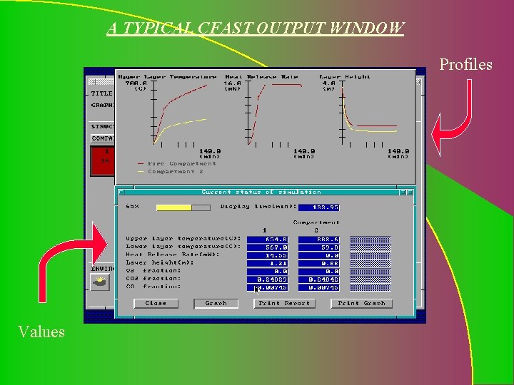
A TYPICAL CFAST OUTPUT WINDOW Profiles Values

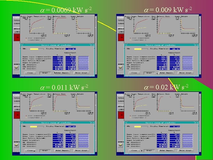
a = 0. 0069 k. W s-2 a = 0. 009 k. W s-2 a = 0. 011 k. W s-2 a = 0. 02 k. W s-2

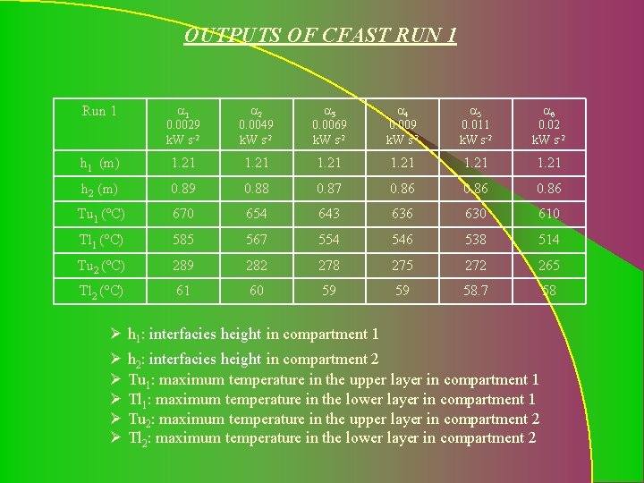
OUTPUTS OF CFAST RUN 1 Run 1 a 1 0. 0029 k. W s-2 a 2 0. 0049 k. W s-2 a 3 0. 0069 k. W s-2 a 4 0. 009 k. W s-2 a 5 0. 011 k. W s-2 a 6 0. 02 k. W s-2 h 1 (m) 1. 21 h 2 (m) 0. 89 0. 88 0. 87 0. 86 Tu 1 (°C) 670 654 643 636 630 610 Tl 1 (°C) 585 567 554 546 538 514 Tu 2 (°C) 289 282 278 275 272 265 Tl 2 (°C) 61 60 59 59 58. 7 58 Ø h 1: interfacies height in compartment 1 Ø h 2: interfacies height in compartment 2 Ø Tu 1: maximum temperature in the upper layer in compartment 1 Ø Tl 1: maximum temperature in the lower layer in compartment 1 Ø Tu 2: maximum temperature in the upper layer in compartment 2 Ø Tl 2: maximum temperature in the lower layer in compartment 2

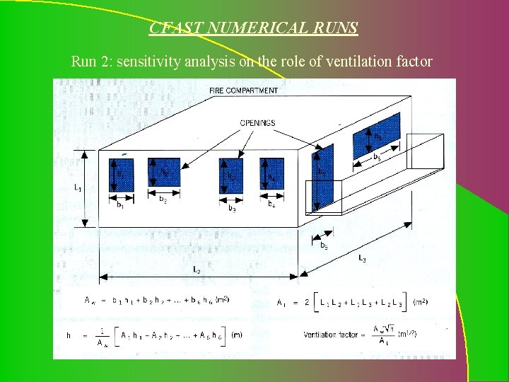
CFAST NUMERICAL RUNS Run 2: sensitivity analysis on the role of ventilation factor

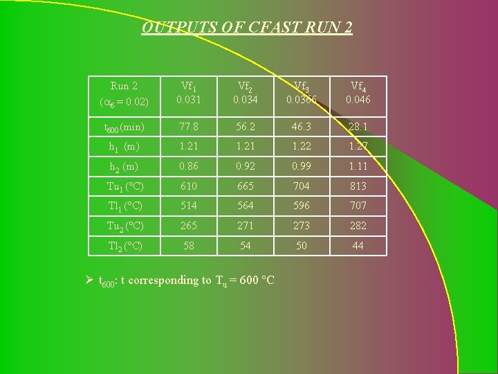
OUTPUTS OF CFAST RUN 2 Run 2 (a 6 = 0. 02) Vf 1 0. 031 Vf 2 0. 034 Vf 3 0. 0366 Vf 4 0. 046 t 600 (min) 77. 8 56. 2 46. 3 28. 1 h 1 (m) 1. 21 1. 22 1. 27 h 2 (m) 0. 86 0. 92 0. 99 1. 11 Tu 1 (°C) 610 665 704 813 Tl 1 (°C) 514 564 596 707 Tu 2 (°C) 265 271 273 282 Tl 2 (°C) 58 54 50 44 Ø t 600: t corresponding to Tu = 600 °C

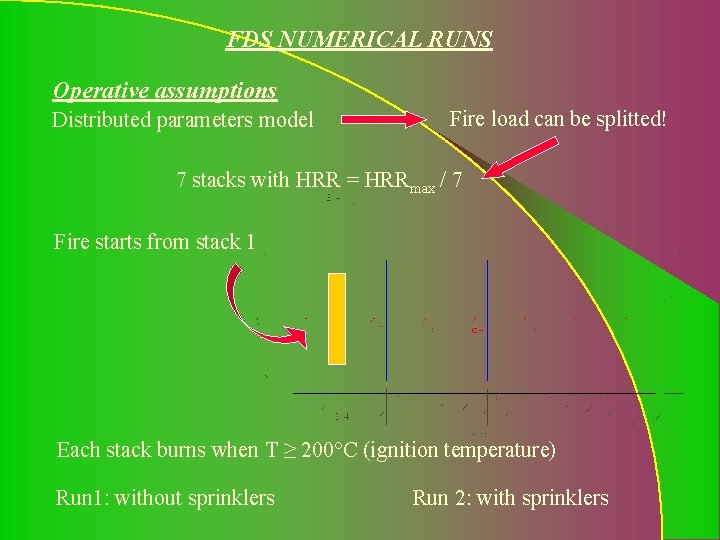
FDS NUMERICAL RUNS Operative assumptions Distributed parameters model Fire load can be splitted! 7 stacks with HRR = HRRmax / 7 Fire starts from stack 1 Each stack burns when T ≥ 200°C (ignition temperature) Run 1: without sprinklers Run 2: with sprinklers

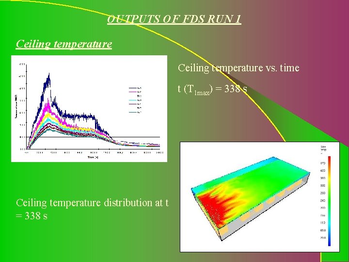
OUTPUTS OF FDS RUN 1 Ceiling temperature vs. time t (T 1 max) = 338 s Ceiling temperature distribution at t = 338 s

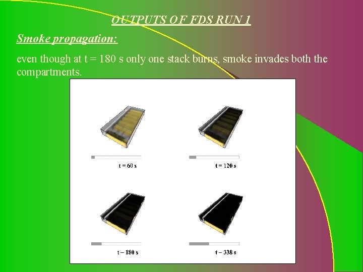
OUTPUTS OF FDS RUN 1 Smoke propagation: even though at t = 180 s only one stack burns, smoke invades both the compartments.

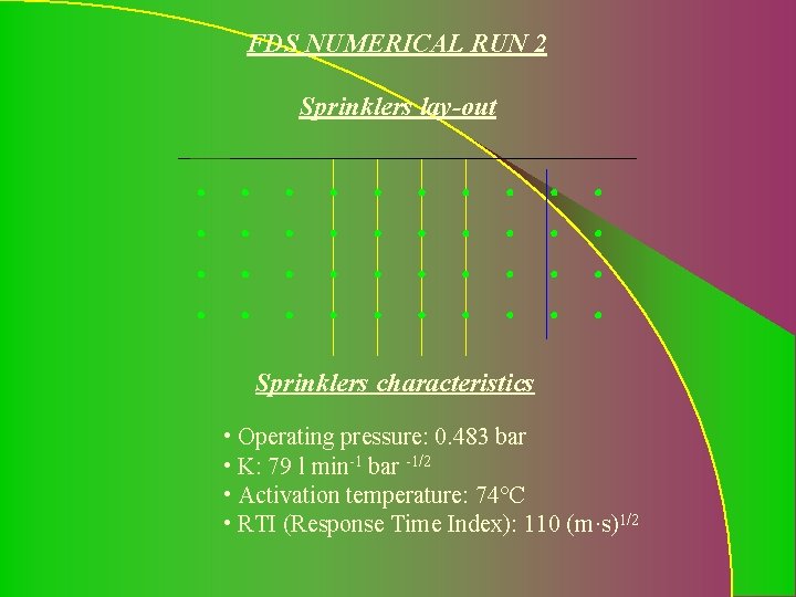
FDS NUMERICAL RUN 2 Sprinklers lay-out Sprinklers characteristics • Operating pressure: 0. 483 bar • K: 79 l min-1 bar -1/2 • Activation temperature: 74°C • RTI (Response Time Index): 110 (m·s)1/2

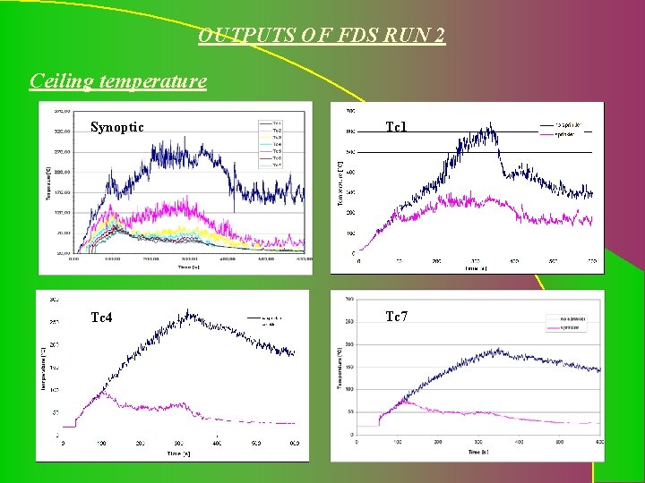
OUTPUTS OF FDS RUN 2 Ceiling temperature Synoptic Tc 1 Tc 4 Tc 7

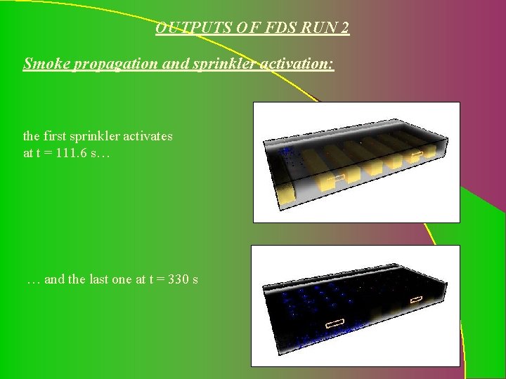
OUTPUTS OF FDS RUN 2 Smoke propagation and sprinkler activation: the first sprinkler activates at t = 111. 6 s… … and the last one at t = 330 s

CONCLUSIONS… • Zone models are very sensitive to ventilation factor and HRR vs. time curve (controlling parameters): they are quick and simple • Field models allow a more realistic and flexible problem description: accurate input estimation is required and simulations are very time expensive • T vs. t curves yielded by the two models are different but similarly shaped … AND FURTHER INVESTIGATIONS • A set of numerical runs has to be carried out in order to gain a deeper insight in T vs. t curves • A comparison between model prediction and deterministic approach results can be performed