MarginSparsity Tradeoff for the Set Covering Machine ECML

Margin-Sparsity Trade-off for the Set Covering Machine ECML 2005 François Laviolette Mario Marchand Mohak Shah (Université Laval) (Université d’Ottawa)

PLAN o Margin-Sparsity trade-off for Sample Compressed Classifiers o The “classical” Set Covering Machine (Classical-SCM) o o The modified Set Covering Machine (SCM 2) o o o Definition Tight Risk Bound and model selection The learning algorithm Definition A non trivial Margin-Sparsity trade-off expressed by the risk bound The learning algorithm Empirical results Conclusions

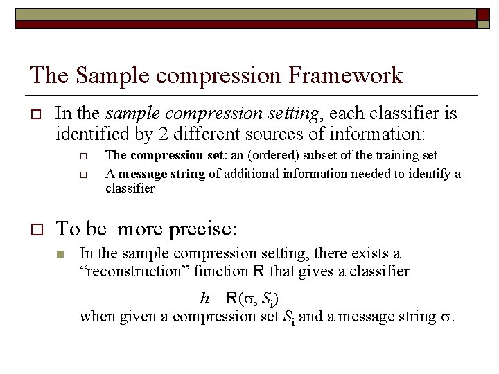
The Sample compression Framework o In the sample compression setting, each classifier is identified by 2 different sources of information: o o o The compression set: an (ordered) subset of the training set A message string of additional information needed to identify a classifier To be more precise: n In the sample compression setting, there exists a “reconstruction” function R that gives a classifier h = R( , Si) when given a compression set Si and a message string .

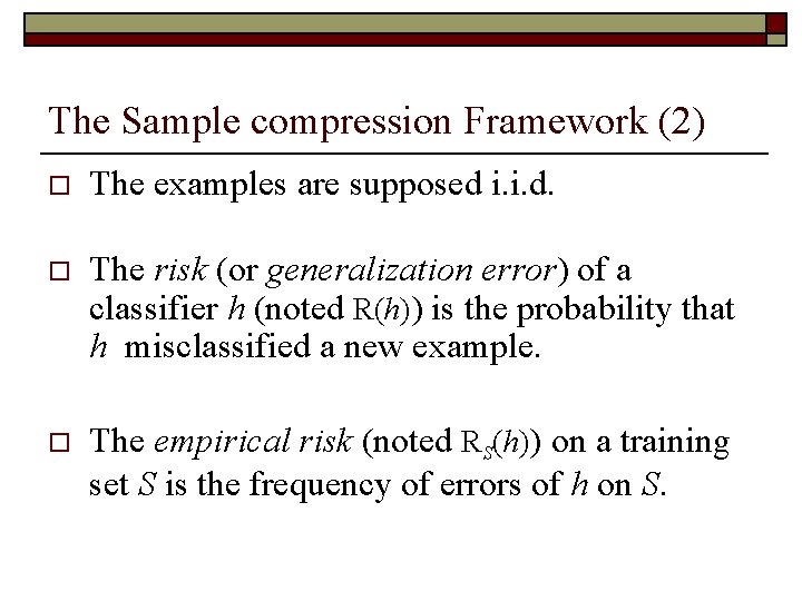
The Sample compression Framework (2) o The examples are supposed i. i. d. o The risk (or generalization error) of a classifier h (noted R(h)) is the probability that h misclassified a new example. o The empirical risk (noted RS(h)) on a training set S is the frequency of errors of h on S.

Examples of sample-compressed classifiers n Set Covering Machines (SCM) [Marchand Shaw-Taylor JMLR 2002] n Decision List Machines (DLM) [Marchand Sokolova JMLR 2005] n Support Vector Machines (SVM) n …

Margin-Sparsity trade-off o There is a widespread belief that in the sample compression setting learning algorithms should somehow try to find a non -trivial margin-sparsity trade-off. o SVM are looking for Margin. n n o But some efforts as been done in order to find a sparser SVM (Bennett (1999), and Bi et al. (2003)). This seems a difficult task. SCM are looking for Sparsity. n n To force a classifier which is a conjunction of “geometric” Boolean features to have no training example within a distance of its decision surface seems a much easier task. Moreover, we will see that in our setting, both sparsity and margin can be considered as different forms of data-compression

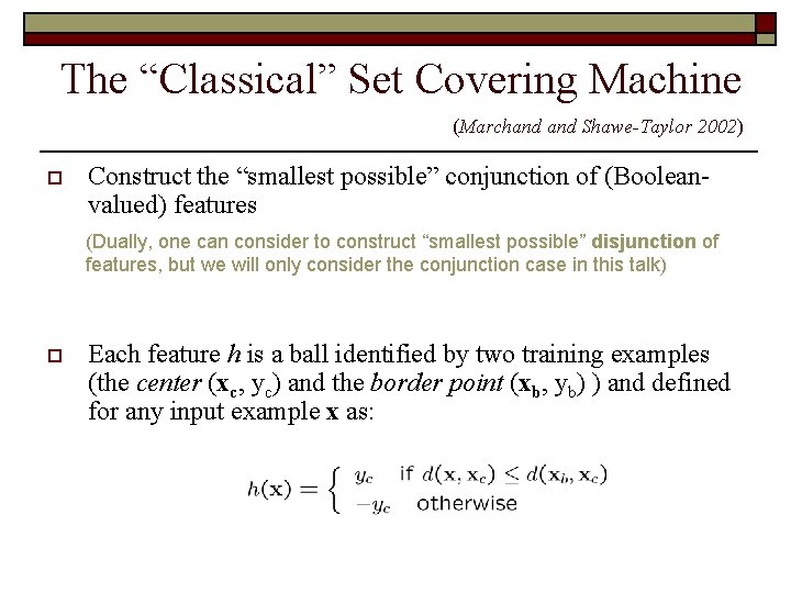
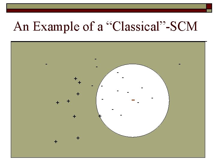
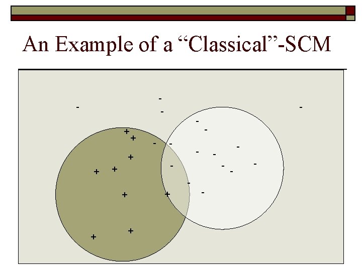
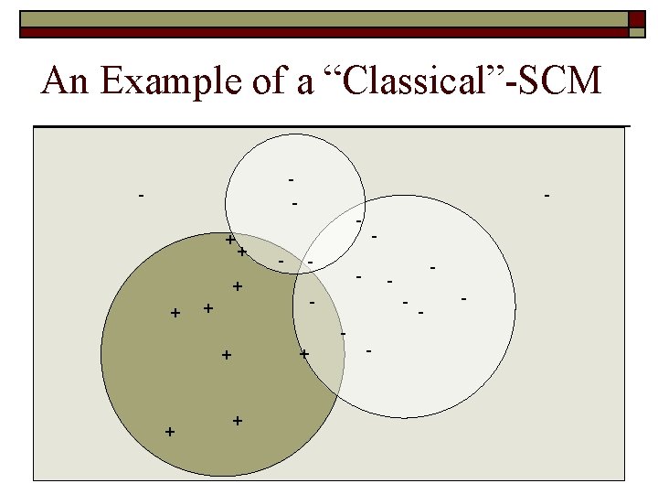
The “Classical” Set Covering Machine (Marchand Shawe-Taylor 2002) o Construct the “smallest possible” conjunction of (Booleanvalued) features (Dually, one can consider to construct “smallest possible” disjunction of features, but we will only consider the conjunction case in this talk) o Each feature h is a ball identified by two training examples (the center (xc, yc) and the border point (xb, yb) ) and defined for any input example x as:

An Example of a “Classical”-SCM - + + - - + + + - - - -

An Example of a “Classical”-SCM - + + - - + + + - - - -

An Example of a “Classical”-SCM - + + + - - - -- -

An Example of a “Classical”-SCM - + + + - - -

An Example of a “Classical”-SCM - + + - - + + + - - - -

An Example of a “Classical”-SCM - + + - - + + + - - - -

An Example of a “Classical”-SCM - + + - - + + + - - - -

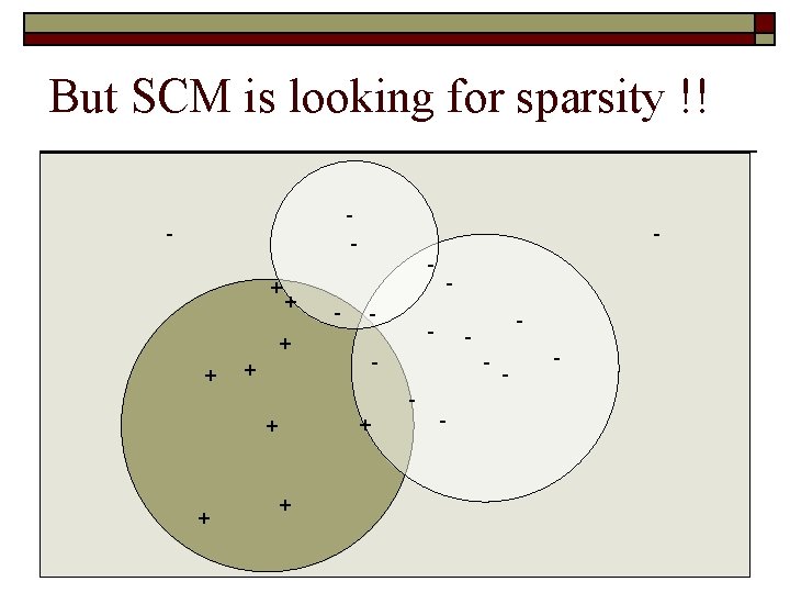
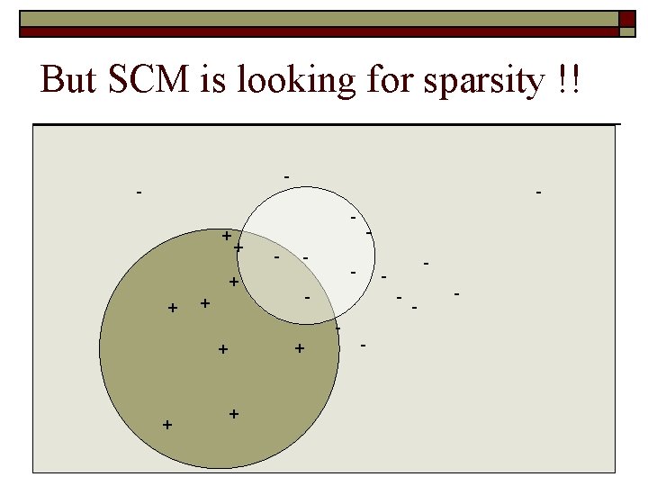
But SCM is looking for sparsity !! - + + - - + + + - - - -

But SCM is looking for sparsity !! - - - + + + - - - -

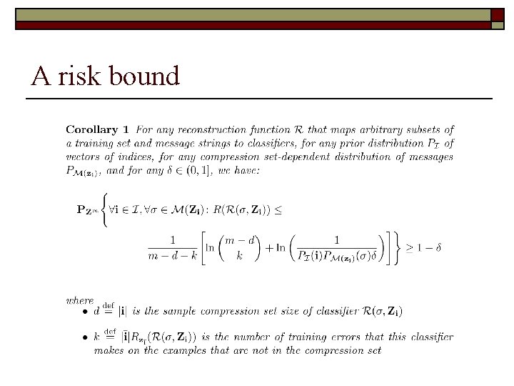
A risk bound

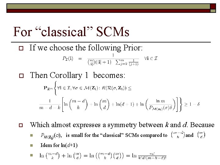
For “classical” SCMs o If we choose the following Prior: o Then Corollary 1 becomes: o Which almost expresses a symmetry between k and d. Because n PM (Z )( ), is small for the “classical” SCMs compared to n Idem for ln(d+1) n i and

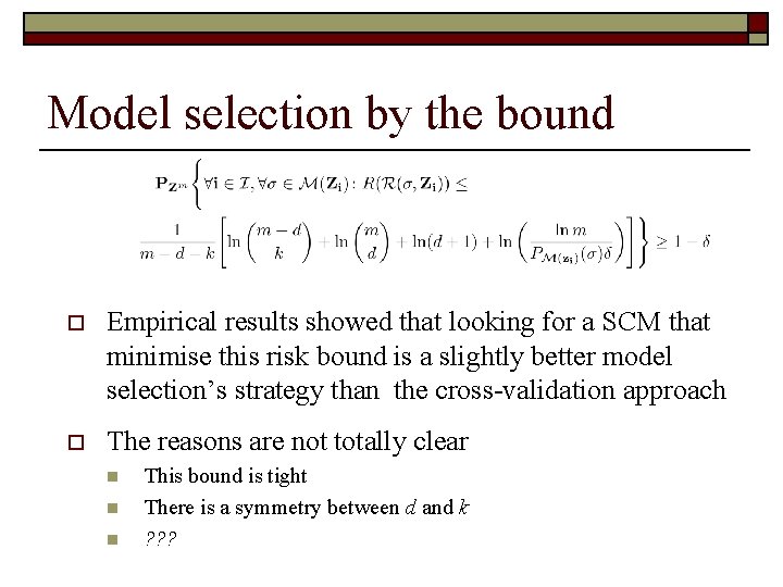
Model selection by the bound o Empirical results showed that looking for a SCM that minimise this risk bound is a slightly better model selection’s strategy than the cross-validation approach o The reasons are not totally clear n n n This bound is tight There is a symmetry between d and k ? ? ?

A Learning algorithm for the “Classical” SCM o Ideally we would like a to find a SCM that minimizes the risk bound o Unfortunately, this is NP-Hard (at least) o We will therefore use a greedy heuristic based on the following observation

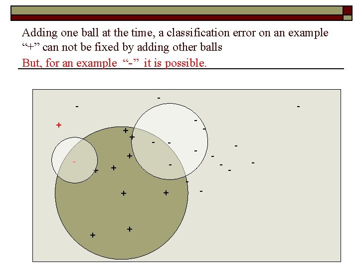
Adding one ball at the time, a classification error on an example “+” can not be fixed by adding other balls But, for an example “-” it is possible. - - - + + + - - - - -

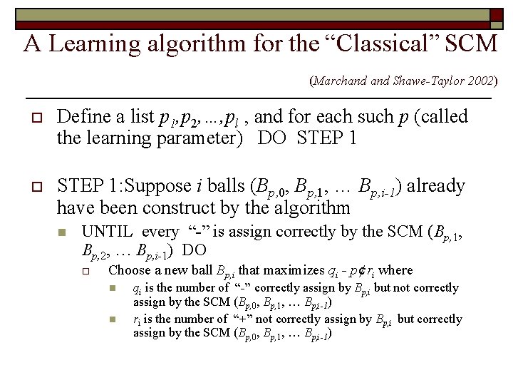
A Learning algorithm for the “Classical” SCM (Marchand Shawe-Taylor 2002) o Define a list p 1, p 2, …, pl , and for each such p (called the learning parameter) DO STEP 1 o STEP 1: Suppose i balls (Bp, 0, Bp, 1, … Bp, i-1) already have been construct by the algorithm n UNTIL every “-” is assign correctly by the SCM (Bp, 1, Bp, 2, … Bp, i-1) DO o Choose a new ball Bp, i that maximizes qi - p ¢ ri where n n qi is the number of “-” correctly assign by Bp, i but not correctly assign by the SCM (Bp, 0, Bp, 1, … Bp, i-1) ri is the number of “+” not correctly assign by Bp, i but correctly assign by the SCM (Bp, 0, Bp, 1, … Bp, i-1)

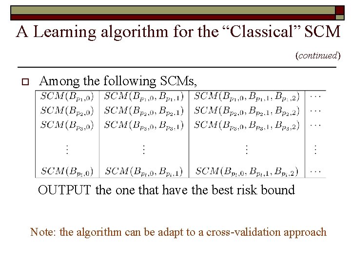
A Learning algorithm for the “Classical” SCM (continued) o Among the following SCMs, OUTPUT the one that have the best risk bound Note: the algorithm can be adapt to a cross-validation approach

SCM 2, SCM with radii coded by message strings o In the “classical” SCM: centers and radii are defined by examples of training set o Another alternative: to code each radius value by a message string (but still use examples of the training set to define the centers) o Objective: to construct the “smallest possible” conjunction of balls each of which having the “smallest possible” number of bits in the message string that define its radius

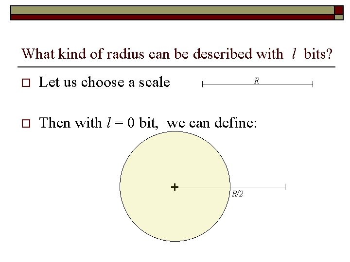
What kind of radius can be described with l bits? o Let us choose a scale o Then with l = 0 bit, we can define: R + R/2

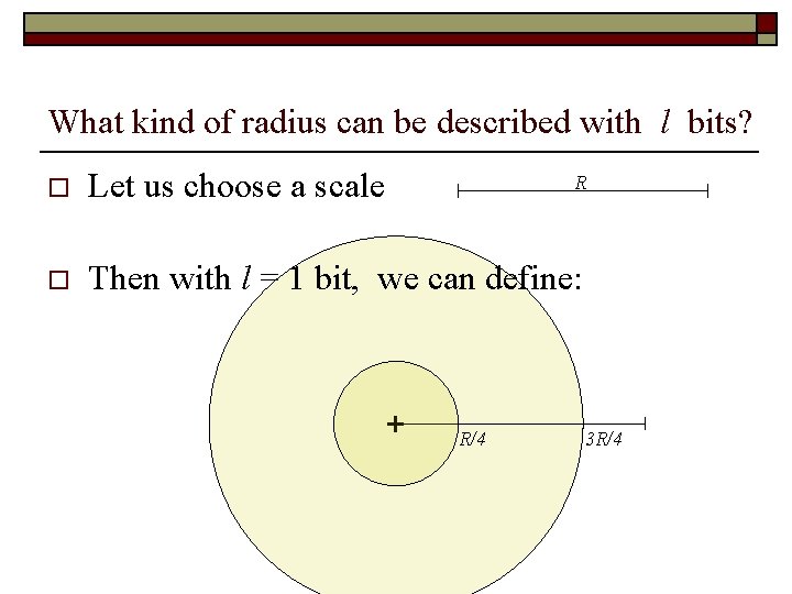
What kind of radius can be described with l bits? o Let us choose a scale o Then with l = 1 bit, we can define: R + R/4 3 R/4

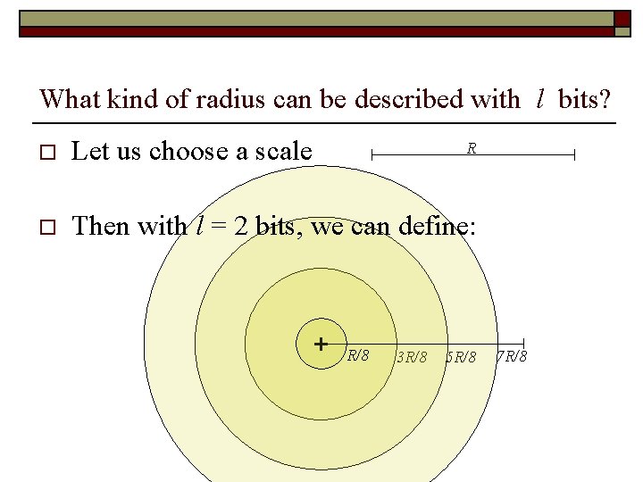
What kind of radius can be described with l bits? o Let us choose a scale o Then with l = 2 bits, we can define: R + R/8 3 R/8 5 R/8 7 R/8

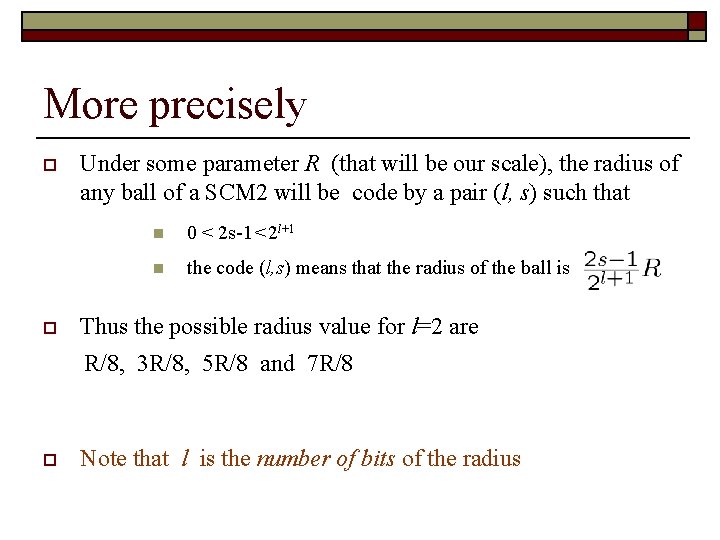
More precisely o o Under some parameter R (that will be our scale), the radius of any ball of a SCM 2 will be code by a pair (l, s) such that n 0 < 2 s-1 < 2 l+1 n the code (l, s) means that the radius of the ball is Thus the possible radius value for l=2 are R/8, 3 R/8, 5 R/8 and 7 R/8 o Note that l is the number of bits of the radius

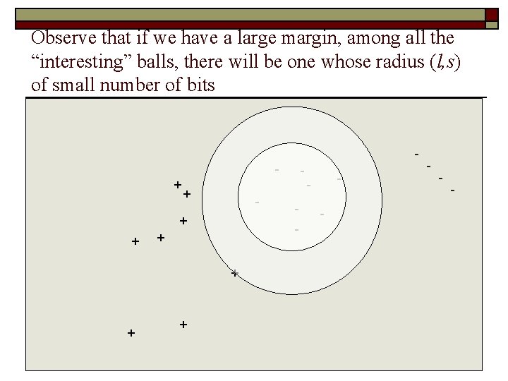
Observe that if we have a large margin, among all the “interesting” balls, there will be one whose radius (l, s) of small number of bits + + - + + + - - - -

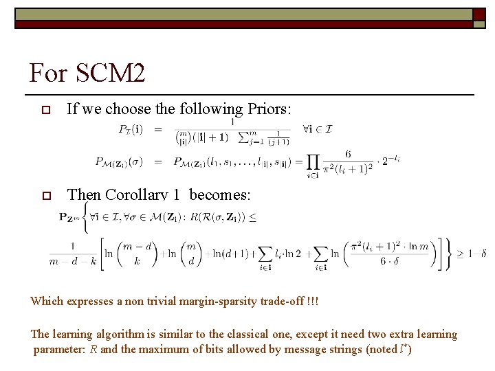
For SCM 2 o If we choose the following Priors: o Then Corollary 1 becomes: Which expresses a non trivial margin-sparsity trade-off !!! The learning algorithm is similar to the classical one, except it need two extra learning parameter: R and the maximum of bits allowed by message strings (noted l*)

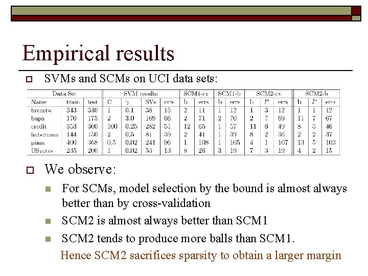
Empirical results o SVMs and SCMs on UCI data sets: o We observe: n n n For SCMs, model selection by the bound is almost always better than by cross-validation SCM 2 is almost always better than SCM 1 SCM 2 tends to produce more balls than SCM 1. Hence SCM 2 sacrifices sparsity to obtain a larger margin

Conclusion We have proposed: o A new representation for the SCM that use two distinct sources of information: n n o A compression set to represent the centers of the balls A message string to encode the radius value of each ball A general data-compression risk bound that depend explicitly on these two information sources which n n exhibits a non trivial trade-off between sparsity (the inverse of the compression set size) and the margin (the inverse of the message length) Seems to be an effective guide for choosing the proper margin-sparsity tradeoff of a classifier