MANOVA Dig it Anova vs Manova Why not

MANOVA Dig it!

Anova vs. Manova • Why not multiple Anovas? • Anovas run separately cannot take into account the pattern of covariation among the dependent measures ▫ It may be possible that multiple Anovas may show no differences while the Manova brings them out ▫ MANOVA is sensitive not only to mean differences but also to the direction and size of correlations among the dependents

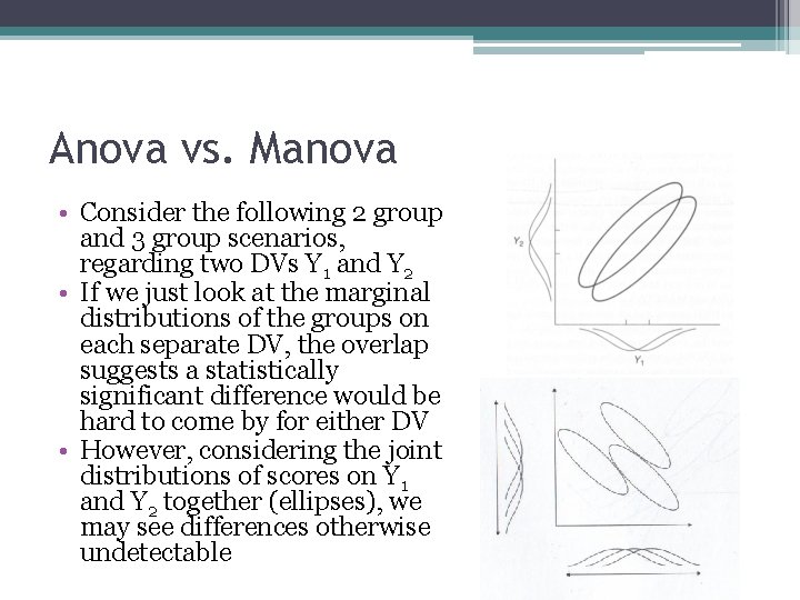
Anova vs. Manova • Consider the following 2 group and 3 group scenarios, regarding two DVs Y 1 and Y 2 • If we just look at the marginal distributions of the groups on each separate DV, the overlap suggests a statistically significant difference would be hard to come by for either DV • However, considering the joint distributions of scores on Y 1 and Y 2 together (ellipses), we may see differences otherwise undetectable

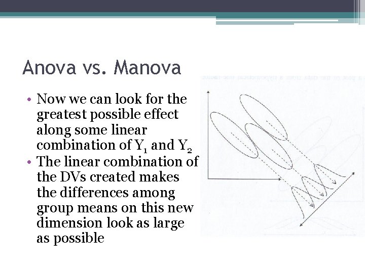
Anova vs. Manova • Now we can look for the greatest possible effect along some linear combination of Y 1 and Y 2 • The linear combination of the DVs created makes the differences among group means on this new dimension look as large as possible

Anova vs. Manova • So, by measuring multiple DVs you increase your chances for finding a group difference ▫ In this sense, in many cases such a test has more power than the univariate procedure, but this is not necessarily true as some seem to believe • Also conducting multiple ANOVAs increases the chance for type 1 error and MANOVA can in some cases help control for the inflation

Kinds of research questions • Which DVs are contributing most to the difference seen on the linear combination of the DVs? � Discriminant analysis • As mentioned, the Manova regards the linear combination of DVs, the individual Anovas do not take into account DV interrelationships • If you are really interested in group differences on the individual DVs, then Manova is not appropriate

Different Multivariate test criteria • • Hotelling’s Trace Wilk’s Lambda, Pillai’s Trace Roy’s Largest Root • What’s going on here? Which to use?

The Multivariate Test of Significance • Thinking in terms of an F statistic, how is the typical F calculated in an Anova calculated? • As a ratio of B/W (actually mean b/t sums of squares and within sums of squares) • Doing so with matrices involves calculating* BW-1 • We take the between subjects matrix and post multiply by the inverted error matrix

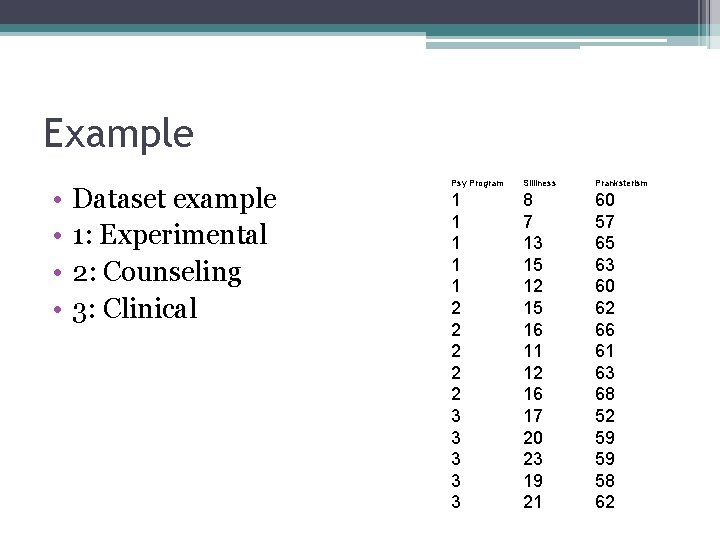
Example • • Dataset example 1: Experimental 2: Counseling 3: Clinical Psy Program Silliness Pranksterism 1 1 1 2 2 2 3 3 3 8 7 13 15 12 15 16 11 12 16 17 20 23 19 21 60 57 65 63 60 62 66 61 63 68 52 59 59 58 62

Example B matrix W matrix • To find the inverse of a matrix one must find the matrix such that A-1 A = I where I is the identity matrix ▫ 1 s on the diagonal, 0 s on the off diagonal • For a two by two matrix it’s not too bad

Example • We find the inverse by first finding the determinate of the original matrix and multiply its inverse by the ‘adjoint’ of that matrix of interest* • Our determinate here is 4688 and so our result for W-1 is You might for practice verify that multiplying this matrix by W will result in a matrix of 1 s on the diagonal and zeros off-diagonal

Example • With this new matrix BW-1, we could find the eigenvalues and eigenvectors associated with it. * • For more detail and a different understanding of what we’re doing, click the icon; for some the detail helps. • For the more practically minded just see the R code below • The eigenvalues of BW-1 are (rounded): ▫ 10. 179 and 0. 226

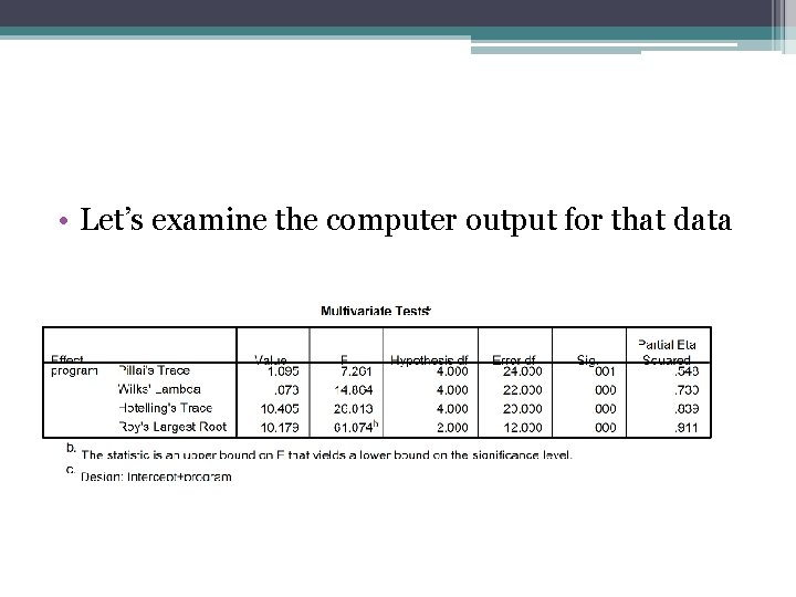
• Let’s examine the computer output for that data

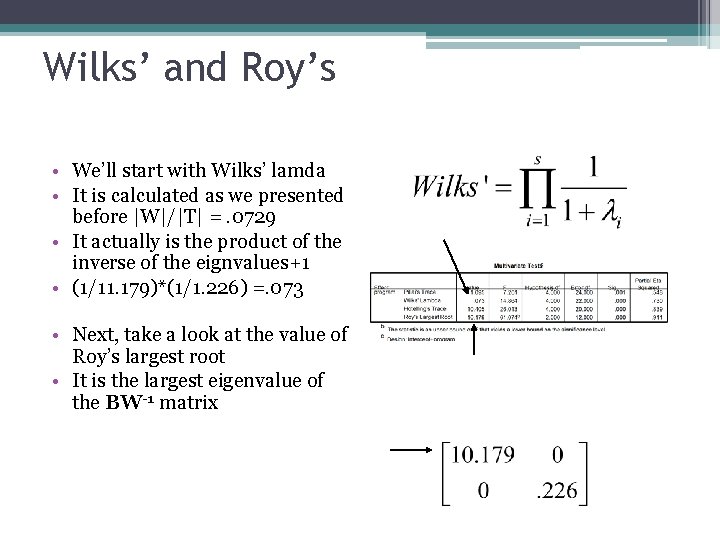
Wilks’ and Roy’s • We’ll start with Wilks’ lamda • It is calculated as we presented before |W|/|T| =. 0729 • It actually is the product of the inverse of the eignvalues+1 • (1/11. 179)*(1/1. 226) =. 073 • Next, take a look at the value of Roy’s largest root • It is the largest eigenvalue of the BW-1 matrix

Pillai’s and Hotelling’s • Pillai’s trace is actually the total of our eigenvalues for the B(B+W)-1 matrix* ▫ Essentially the sum of the variance accounted in the variates • Here we see it is the sum of the eigenvalue/1+eigenvalue ratios ▫ 10. 179/11. 179 +. 226/1. 226 = 1. 095 • Now look at Hotelling’s Trace • It is simply the sum of the eigenvalues of our ▫ 10. 179 +. 226 = 10. 405

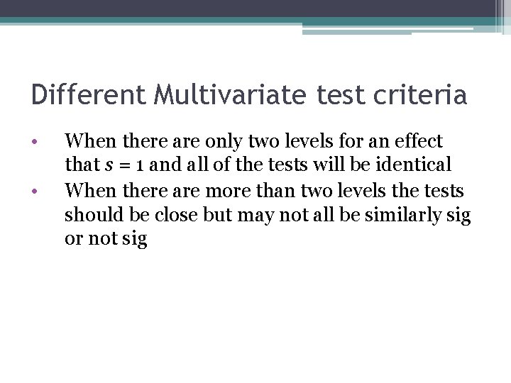
Different Multivariate test criteria • • When there are only two levels for an effect that s = 1 and all of the tests will be identical When there are more than two levels the tests should be close but may not all be similarly sig or not sig

Different Multivariate test criteria • • • As we saw, when there are more than two levels there are multiple ways in which the data can be combined to separate the groups Wilk’s Lambda, Hotelling’s Trace and Pillai’s trace all pool the variance from all the dimensions to create the test statistic. Roy’s largest root only uses the variance from the dimension that separates the groups most (the largest “root” or difference).

Which do you choose? • • • ▫ • Wilks’ lambda is the traditional choice, and most widely used Wilks’, Hotelling’s, and Pillai’s have shown to be robust (type I sense) to problems with assumptions (e. g. violation of homogeneity of covariances), Pillai’s more so, but it is also the most conservative usually. Roy’s is the more liberal test usually (though none are always most powerful), but it loses its strength when the differences lie along more than one dimension Some packages will even not provide statistics associated with it However in practice differences are often seen mostly along one dimension, and Roy’s is usually more powerful in that case (if Ho. Cov assumption is met)

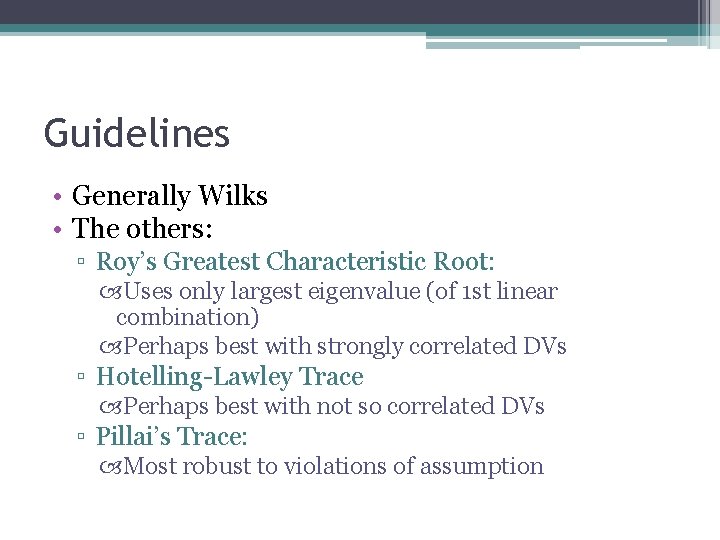
Guidelines • Generally Wilks • The others: ▫ Roy’s Greatest Characteristic Root: Uses only largest eigenvalue (of 1 st linear combination) Perhaps best with strongly correlated DVs ▫ Hotelling-Lawley Trace Perhaps best with not so correlated DVs ▫ Pillai’s Trace: Most robust to violations of assumption

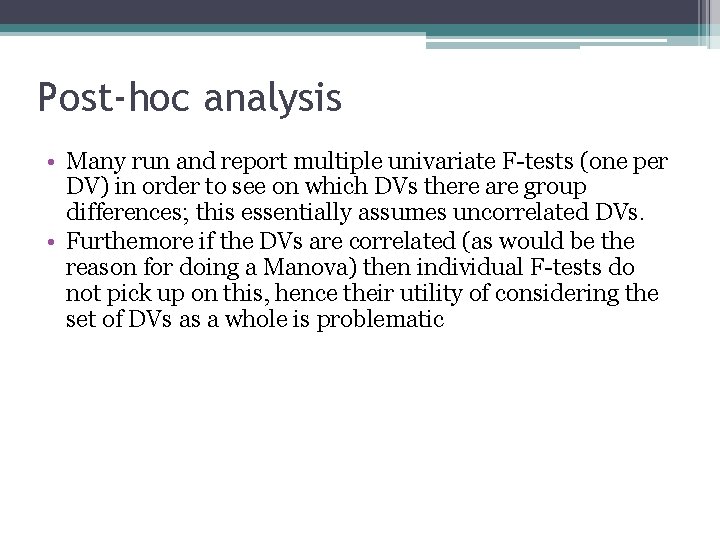
Post-hoc analysis • Many run and report multiple univariate F-tests (one per DV) in order to see on which DVs there are group differences; this essentially assumes uncorrelated DVs. • Furthemore if the DVs are correlated (as would be the reason for doing a Manova) then individual F-tests do not pick up on this, hence their utility of considering the set of DVs as a whole is problematic

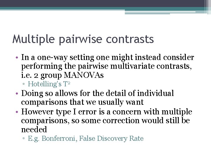
Multiple pairwise contrasts • In a one-way setting one might instead consider performing the pairwise multivariate contrasts, i. e. 2 group MANOVAs ▫ Hotelling’s T 2 • Doing so allows for the detail of individual comparisons that we usually want • However type I error is a concern with multiple comparisons, so some correction would still be needed ▫ E. g. Bonferroni, False Discovery Rate

Assessing DV importance • Our previous discussion focused on group differences • We might instead or also be interest in individual DV contribution to the group differences • While in some cases univariate analyses may reflect DV importance in the multivariate analysis, better methods/approaches are available

Discriminant Function Analysis • It uses group membership as the DV and the Manova DVs as predictors of group membership* • Using this as a follow up to MANOVA will give you the relative importance of each DV predicting group membership (in a multiple regression sense)

DFA • Some suggest that interpreting the correlations of the p variables and the discriminant function (i. e. their loadings as we called them for cancorr) as studies suggest they are more stable from sample to sample • So while the weights give an assessment of unique contribution, the loadings can give a sense of how much correlation a variable has with the underlying composite