Managerial Economics Dr Nihal Hennayake What is Microeconomics

Managerial Economics Dr Nihal Hennayake

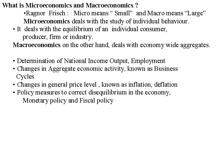
What is Microeconomics and Macroeconomics ? • Ragnor Frisch : Micro means “ Small” and Macro means “Large” Microeconomics deals with the study of individual behaviour. • It deals with the equilibrium of an individual consumer, producer, firm or industry. Macroeconomics on the other hand, deals with economy wide aggregates. • Determination of National Income Output, Employment • Changes in Aggregate economic activity, known as Business Cycles • Changes in general price level , known as inflation, deflation • Policy measures to correct disequilibrium in the economy, Monetary policy and Fiscal policy

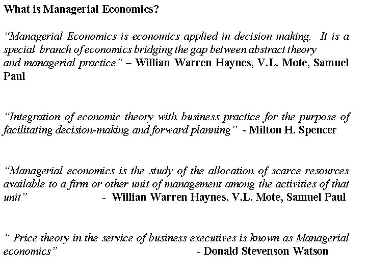
What is Managerial Economics? “Managerial Economics is economics applied in decision making. It is a special branch of economics bridging the gap between abstract theory and managerial practice” – Willian Warren Haynes, V. L. Mote, Samuel Paul “Integration of economic theory with business practice for the purpose of facilitating decision-making and forward planning” - Milton H. Spencer “Managerial economics is the study of the allocation of scarce resources available to a firm or other unit of management among the activities of that unit” - Willian Warren Haynes, V. L. Mote, Samuel Paul “ Price theory in the service of business executives is known as Managerial economics” - Donald Stevenson Watson

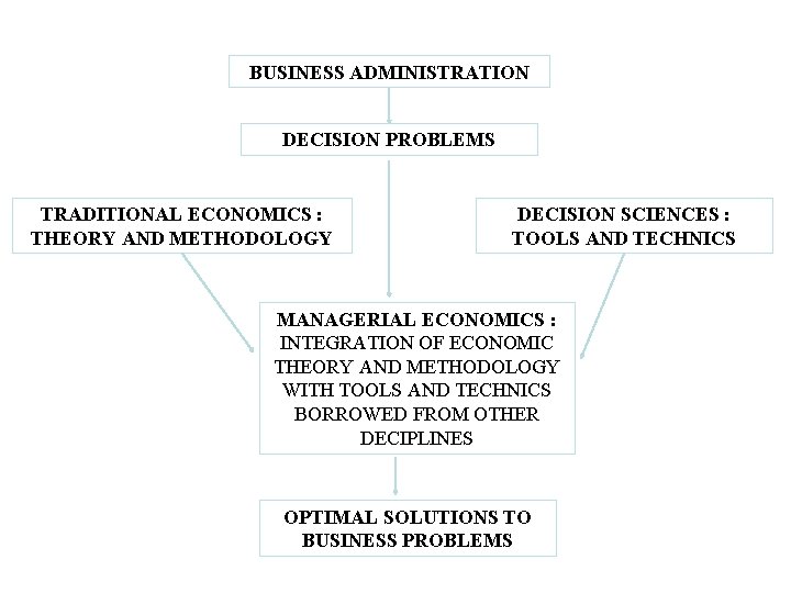
BUSINESS ADMINISTRATION DECISION PROBLEMS TRADITIONAL ECONOMICS : THEORY AND METHODOLOGY DECISION SCIENCES : TOOLS AND TECHNICS MANAGERIAL ECONOMICS : INTEGRATION OF ECONOMIC THEORY AND METHODOLOGY WITH TOOLS AND TECHNICS BORROWED FROM OTHER DECIPLINES OPTIMAL SOLUTIONS TO BUSINESS PROBLEMS

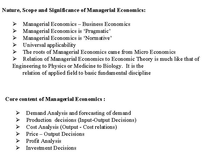
Nature, Scope and Significance of Managerial Economics: Ø Managerial Economics – Business Economics Ø Managerial Economics is ‘Pragmatic’ Ø Managerial Economics is ‘Normative’ Ø Universal applicability Ø The roots of Managerial Economics came from Micro Economics Ø Relation of Managerial Economics to Economic Theory is much like that of Engineering to Physics or Medicine to Biology. It is the relation of applied field to basic fundamental discipline Core content of Managerial Economics : Ø Ø Ø Demand Analysis and forecasting of demand Production decisions (Input-Output Decisions) Cost Analysis (Output - Cost relations) Price – Output Decisions Profit Analysis Investment Decisions

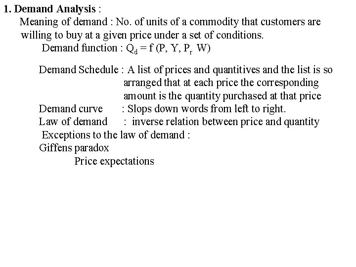
1. Demand Analysis : Meaning of demand : No. of units of a commodity that customers are willing to buy at a given price under a set of conditions. Demand function : Qd = f (P, Y, Pr W) Demand Schedule : A list of prices and quantitives and the list is so arranged that at each price the corresponding amount is the quantity purchased at that price Demand curve : Slops down words from left to right. Law of demand : inverse relation between price and quantity Exceptions to the law of demand : Giffens paradox Price expectations

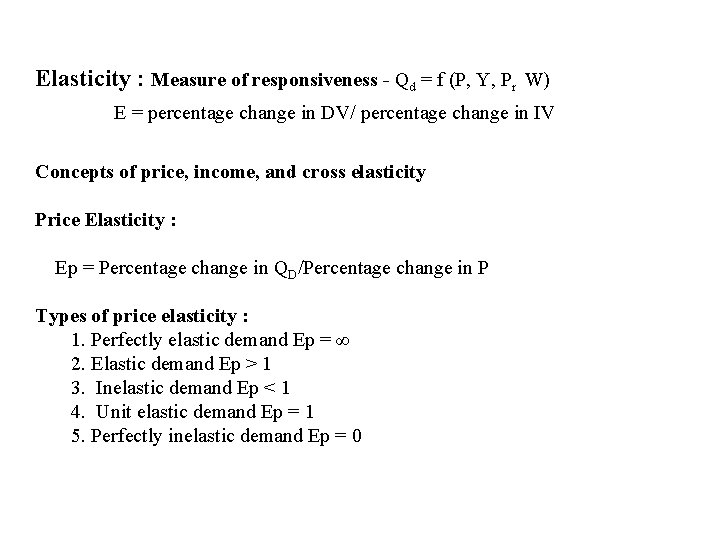
Elasticity : Measure of responsiveness - Qd = f (P, Y, Pr W) E = percentage change in DV/ percentage change in IV Concepts of price, income, and cross elasticity Price Elasticity : Ep = Percentage change in QD/Percentage change in P Types of price elasticity : 1. Perfectly elastic demand Ep = ∞ 2. Elastic demand Ep > 1 3. Inelastic demand Ep < 1 4. Unit elastic demand Ep = 1 5. Perfectly inelastic demand Ep = 0

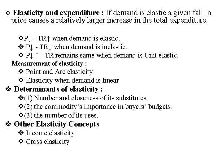
v Elasticity and expenditure : If demand is elastic a given fall in price causes a relatively larger increase in the total expenditure. v. P↓ - TR↑ when demand is elastic. v P↓ - TR↓ when demand is inelastic. v P↓ ↑ - TR remains same when demand is Unit elastic. Measurement of elasticity : v Point and Arc elasticity v Elasticity when demand is linear v Determinants of elasticity : v(1) Number and closeness of its substitutes, v(2) the commodity’s importance in buyers’ budgets, v(3) the number of its uses. v Other Elasticity Concepts v Income elasticity v Cross elasticity

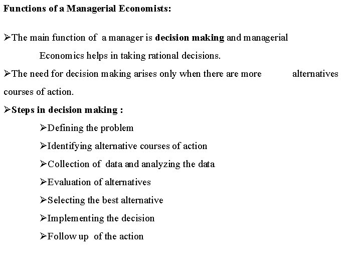
Functions of a Managerial Economists: ØThe main function of a manager is decision making and managerial Economics helps in taking rational decisions. ØThe need for decision making arises only when there are more courses of action. ØSteps in decision making : ØDefining the problem ØIdentifying alternative courses of action ØCollection of data and analyzing the data ØEvaluation of alternatives ØSelecting the best alternative ØImplementing the decision ØFollow up of the action alternatives

Specific functions to be performed by a managerial Economist : 1. Production scheduling 2. Sales forecasting 3. Market research 4. Economic analysis of competing companies 5. Pricing problems of industry 6. Investment appraisal 7. Security analysis 8. Advice on foreign exchange management 9. Advice on trade 10. Environmental forecasting

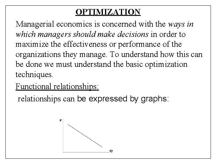
OPTIMIZATION Managerial economics is concerned with the ways in which managers should make decisions in order to maximize the effectiveness or performance of the organizations they manage. To understand how this can be done we must understand the basic optimization techniques. Functional relationships: relationships can be expressed by graphs:

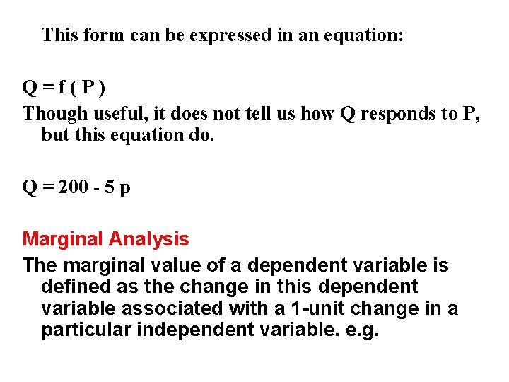
This form can be expressed in an equation: Q=f(P) Though useful, it does not tell us how Q responds to P, but this equation do. Q = 200 - 5 p Marginal Analysis The marginal value of a dependent variable is defined as the change in this dependent variable associated with a 1 -unit change in a particular independent variable. e. g.

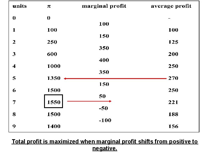
Total profit is maximized when marginal profit shifts from positive to negative.

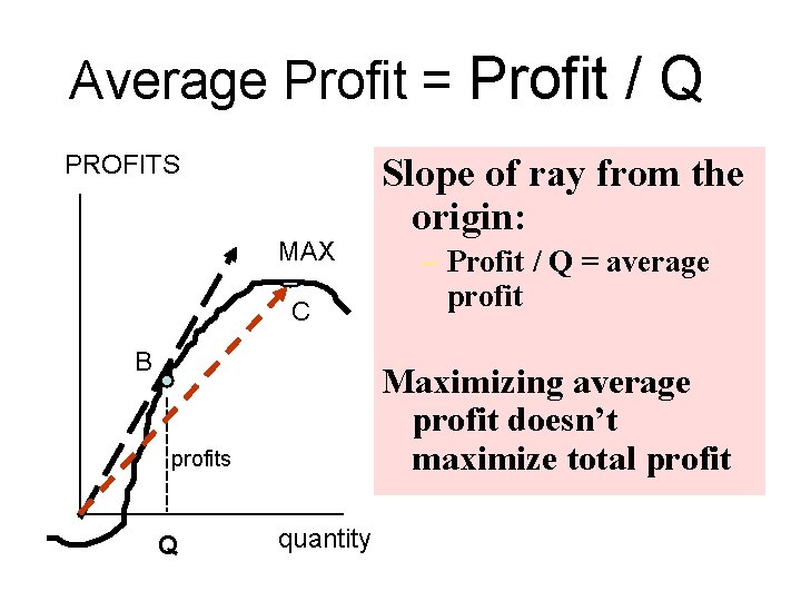
Average Profit = Profit / Q PROFITS MAX C B – Profit / Q = average profit Maximizing average profit doesn’t maximize total profits Q Slope of ray from the origin: quantity

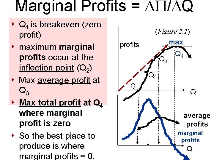
Marginal Profits = / Q s Q 1 is breakeven (zero profit) s maximum marginal profits occur at the inflection point (Q 2) s Max average profit at Q 3 s Max total profit at Q 4 where marginal profit is zero s So the best place to produce is where marginal profits = 0. profits (Figure 2. 1) max Q 3 Q 4 Q 2 Q 1 Q average profits marginal profits Q

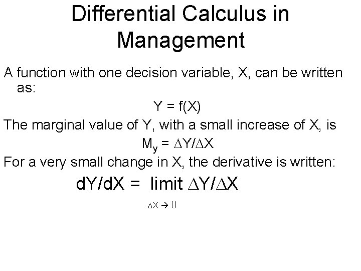
Differential Calculus in Management A function with one decision variable, X, can be written as: Y = f(X) The marginal value of Y, with a small increase of X, is My = Y/ X For a very small change in X, the derivative is written: d. Y/d. X = limit Y/ X X 0

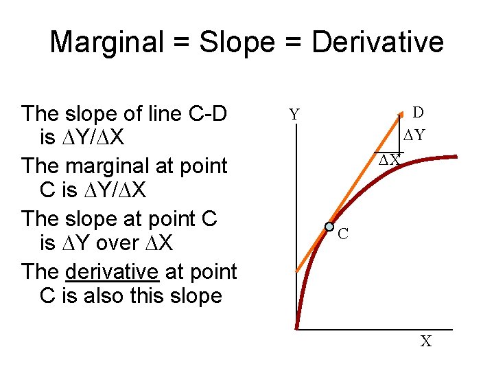
Marginal = Slope = Derivative The slope of line C-D is Y/ X The marginal at point C is Y/ X The slope at point C is Y over X The derivative at point C is also this slope D Y Y X C X

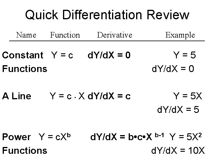
Quick Differentiation Review Name Function Constant Y = c Functions A Line Derivative Example d. Y/d. X = 0 Y=5 d. Y/d. X = 0 Y = c • X d. Y/d. X = c Power Y = c. Xb Functions Y = 5 X d. Y/d. X = 5 d. Y/d. X = b • c • X b-1 Y = 5 X 2 d. Y/d. X = 10 X

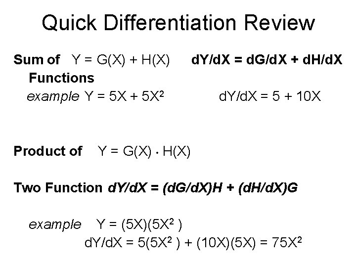
Quick Differentiation Review Sum of Y = G(X) + H(X) Functions example Y = 5 X + 5 X 2 Product of d. Y/d. X = d. G/d. X + d. H/d. X d. Y/d. X = 5 + 10 X Y = G(X) • H(X) Two Function d. Y/d. X = (d. G/d. X)H + (d. H/d. X)G example Y = (5 X)(5 X 2 ) d. Y/d. X = 5(5 X 2 ) + (10 X)(5 X) = 75 X 2

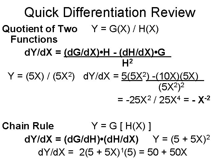
Quick Differentiation Review Quotient of Two Y = G(X) / H(X) Functions d. Y/d. X = (d. G/d. X) • H - (d. H/d. X) • G H 2 Y = (5 X) / (5 X 2) d. Y/d. X = 5(5 X 2) -(10 X)(5 X) (5 X 2)2 = -25 X 2 / 25 X 4 = - X-2 Chain Rule Y = G [ H(X) ] d. Y/d. X = (d. G/d. H) • (d. H/d. X) Y = (5 + 5 X)2 d. Y/d. X = 2(5 + 5 X)1(5) = 50 + 50 X

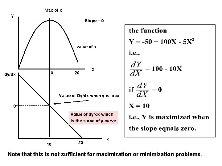
Max of x y Slope = 0 value of x dy/dx 10 20 x Value of Dy/dx when y is max 0 Value of dy/dx which Is the slope of y curve 10 20 x Note that this is not sufficient for maximization or minimization problems.

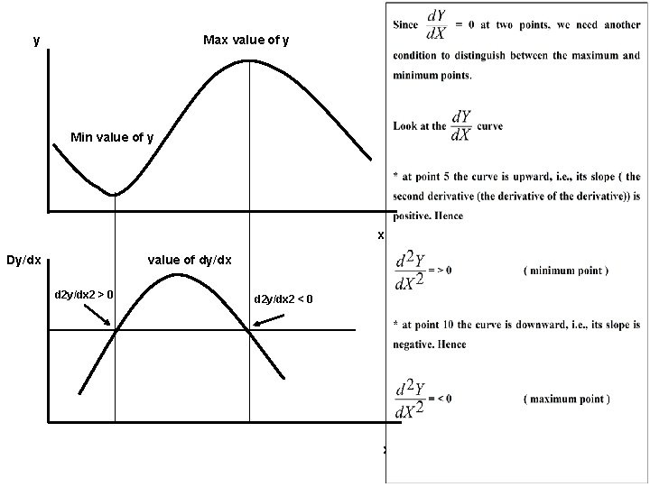
y Max value of y Min value of y x Dy/dx value of dy/dx d 2 y/dx 2 > 0 d 2 y/dx 2 < 0 x

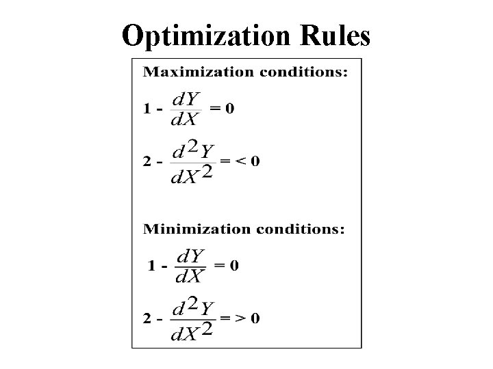
Optimization Rules

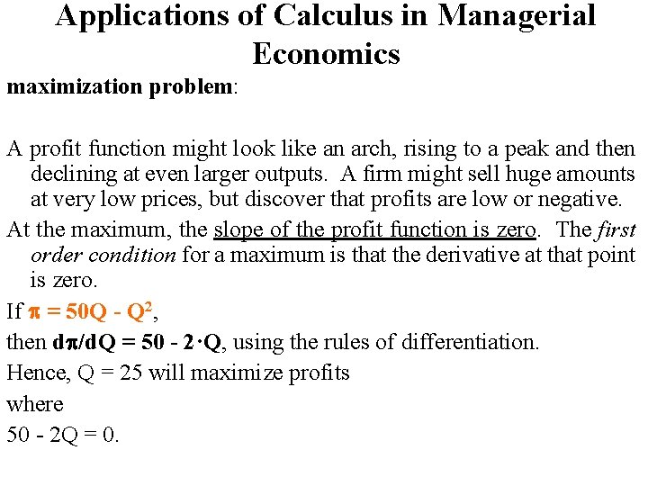
Applications of Calculus in Managerial Economics maximization problem: A profit function might look like an arch, rising to a peak and then declining at even larger outputs. A firm might sell huge amounts at very low prices, but discover that profits are low or negative. At the maximum, the slope of the profit function is zero. The first order condition for a maximum is that the derivative at that point is zero. If = 50 Q - Q 2, then d /d. Q = 50 - 2·Q, using the rules of differentiation. Hence, Q = 25 will maximize profits where 50 - 2 Q = 0.

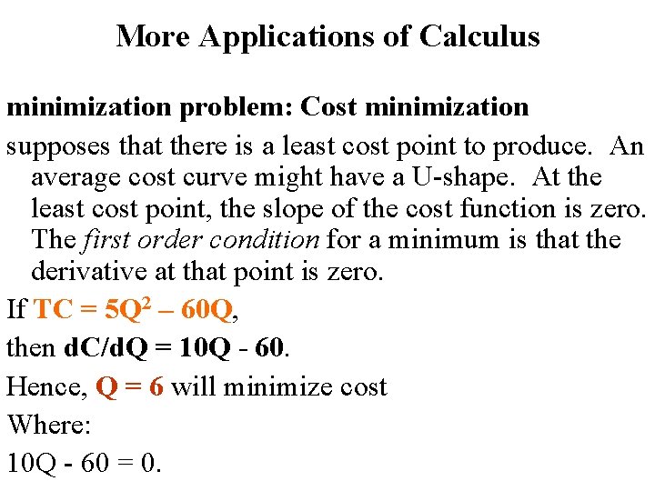
More Applications of Calculus minimization problem: Cost minimization supposes that there is a least cost point to produce. An average cost curve might have a U-shape. At the least cost point, the slope of the cost function is zero. The first order condition for a minimum is that the derivative at that point is zero. If TC = 5 Q 2 – 60 Q, then d. C/d. Q = 10 Q - 60. Hence, Q = 6 will minimize cost Where: 10 Q - 60 = 0.

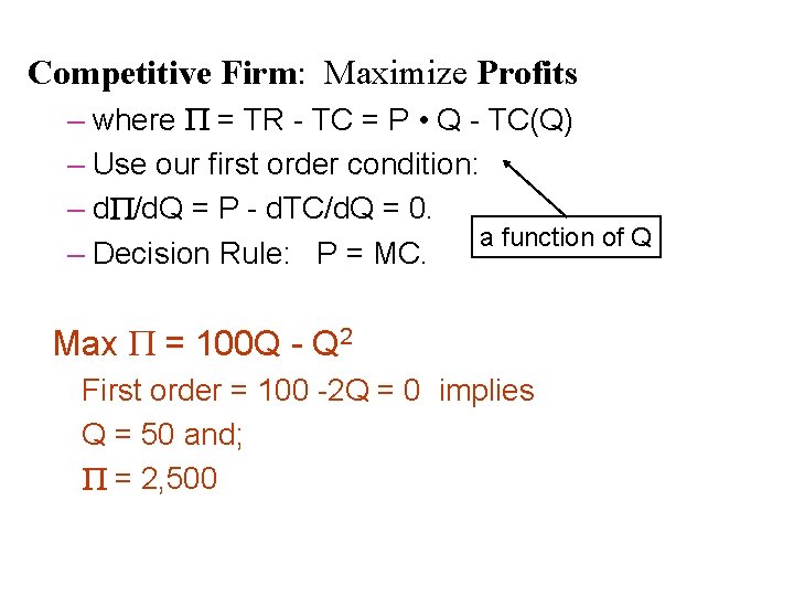
Competitive Firm: Maximize Profits – where = TR - TC = P • Q - TC(Q) – Use our first order condition: – d /d. Q = P - d. TC/d. Q = 0. a function of Q – Decision Rule: P = MC. Max = 100 Q - Q 2 First order = 100 -2 Q = 0 implies Q = 50 and; = 2, 500

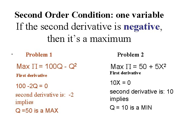
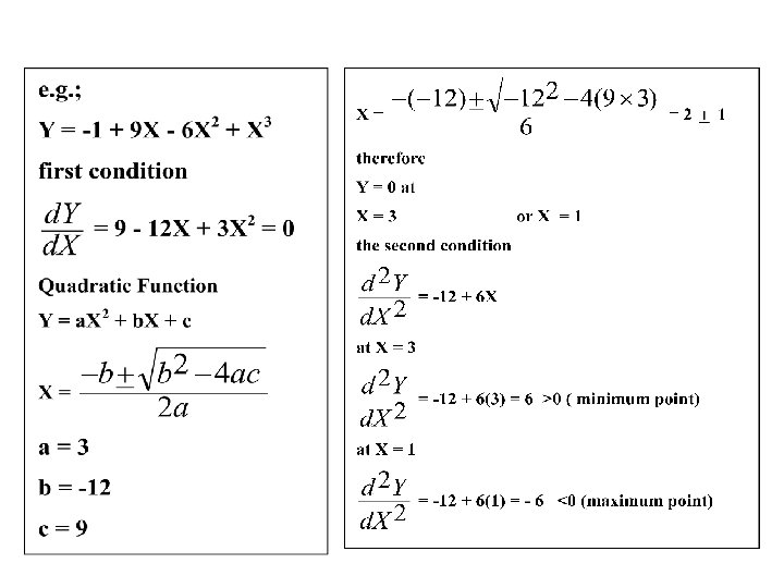
Second Order Condition: one variable If the second derivative is negative, then it’s a maximum. Problem 1 Max = 100 Q - Q 2 First derivative 100 -2 Q = 0 second derivative is: -2 implies Q =50 is a MAX Problem 2 Max = 50 + 5 X 2 First derivative 10 X = 0 second derivative is: 10 implies Q = 10 is a MIN

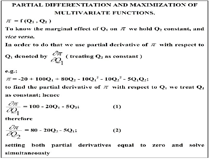
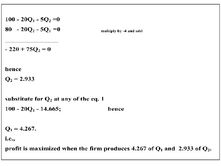
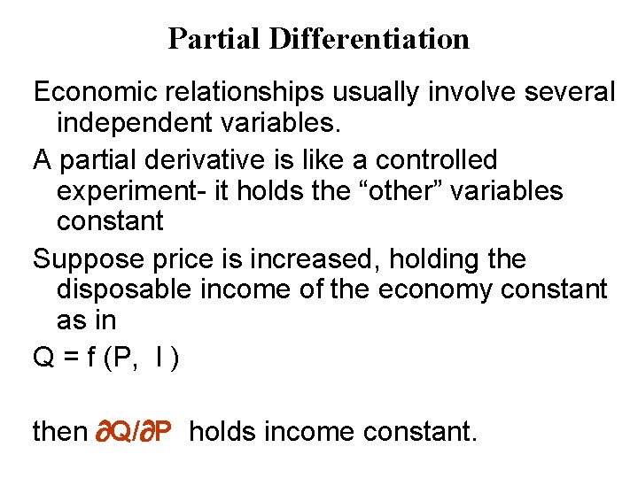
Partial Differentiation Economic relationships usually involve several independent variables. A partial derivative is like a controlled experiment- it holds the “other” variables constant Suppose price is increased, holding the disposable income of the economy constant as in Q = f (P, I ) then Q/ P holds income constant.

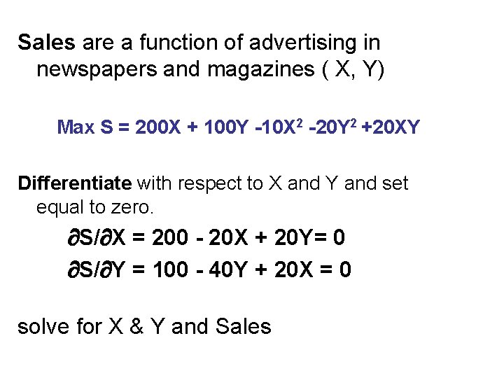
Sales are a function of advertising in newspapers and magazines ( X, Y) Max S = 200 X + 100 Y -10 X 2 -20 Y 2 +20 XY Differentiate with respect to X and Y and set equal to zero. S/ X = 200 - 20 X + 20 Y= 0 S/ Y = 100 - 40 Y + 20 X = 0 solve for X & Y and Sales

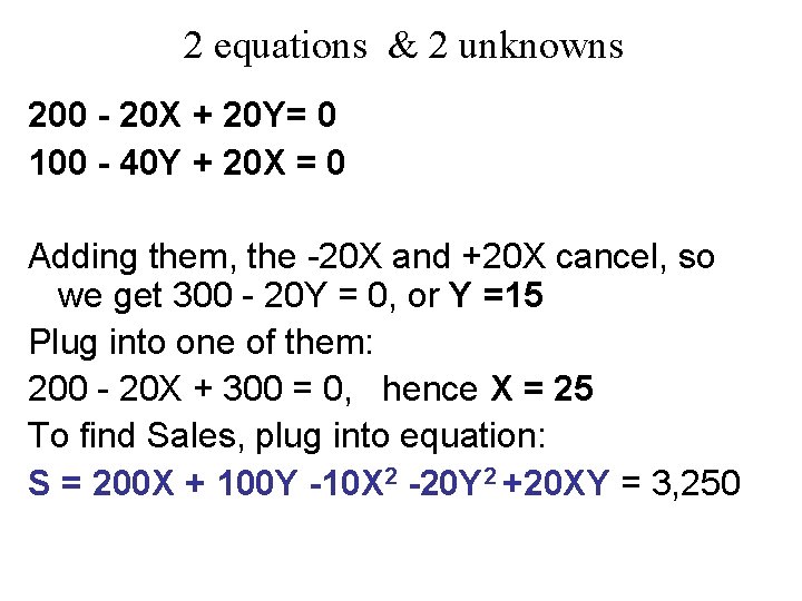
2 equations & 2 unknowns 200 - 20 X + 20 Y= 0 100 - 40 Y + 20 X = 0 Adding them, the -20 X and +20 X cancel, so we get 300 - 20 Y = 0, or Y =15 Plug into one of them: 200 - 20 X + 300 = 0, hence X = 25 To find Sales, plug into equation: S = 200 X + 100 Y -10 X 2 -20 Y 2 +20 XY = 3, 250