Linear Programming Concepts Concepts What is Linear Programming

Linear Programming

Concepts

Concepts What is Linear Programming? Linear programming method is a technique for choosing the best alternative from a set of feasible alternatives, in situations in which the objective function as well as the constraints can be expressed as linear mathematical functions.

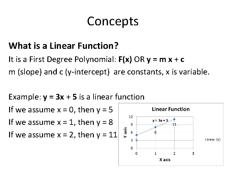
Concepts What is a Linear Function? It is a First Degree Polynomial: F(x) OR y = m x + c m (slope) and c (y-intercept) are constants, x is variable. Example: y = 3 x + 5 is a linear function If we assume x = 0, then y = 5 If we assume x = 1, then y = 8 If we assume x = 2, then y = 11

Concepts Properties of Linear Programming Models: § Seek to minimize or maximize § Include constraints or limitations § There must be alternatives available § All equations are linear

Linear Programming Example

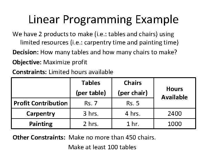
Linear Programming Example We have 2 products to make (i. e. : tables and chairs) using limited resources (i. e. : carpentry time and painting time) Decision: How many tables and how many chairs to make? Objective: Maximize profit Constraints: Limited hours available Profit Contribution Tables (per table) Rs. 7 Chairs (per chair) Rs. 5 Hours Available Carpentry Painting 3 hrs. 2 hrs. 4 hrs. 1 hr. 2400 1000 Other Constraints: Make no more than 450 chairs. Make at least 100 tables

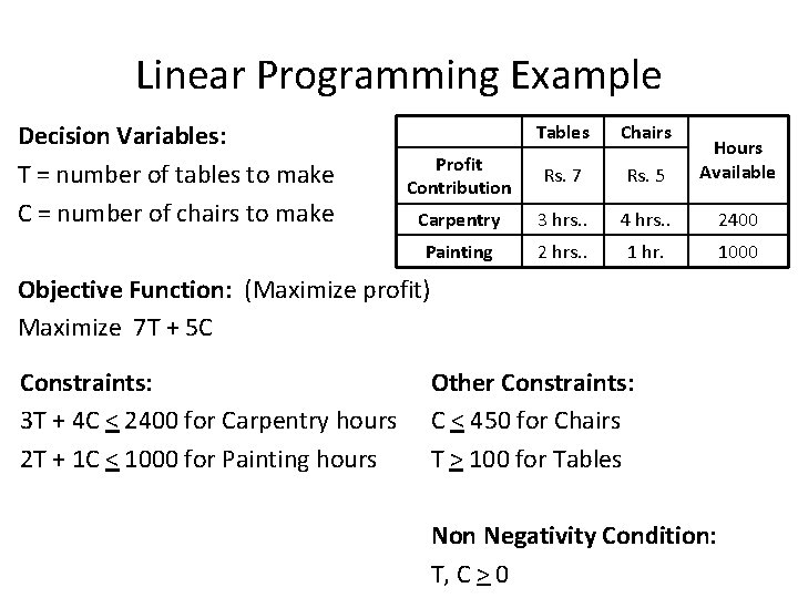
Linear Programming Example Decision Variables: T = number of tables to make C = number of chairs to make Tables Chairs Profit Contribution Rs. 7 Rs. 5 Hours Available Carpentry 3 hrs. . 4 hrs. . 2400 Painting 2 hrs. . 1 hr. 1000 Objective Function: (Maximize profit) Maximize 7 T + 5 C Constraints: 3 T + 4 C < 2400 for Carpentry hours 2 T + 1 C < 1000 for Painting hours Other Constraints: C < 450 for Chairs T > 100 for Tables Non Negativity Condition: T, C > 0

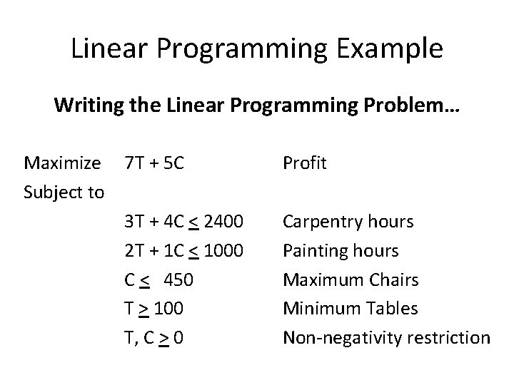
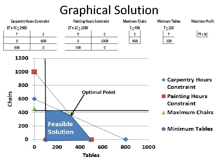
Linear Programming Example Writing the Linear Programming Problem… Maximize 7 T + 5 C Subject to 3 T + 4 C < 2400 2 T + 1 C < 1000 C < 450 T > 100 T, C > 0 Profit Carpentry hours Painting hours Maximum Chairs Minimum Tables Non-negativity restriction

Linear Programming Example Graphical Solution* * can only be done in 2 dimensions

Characteristics of Linear Programming Graphical Method • Feasible Region: The set of points that satisfies all constraints • Corner Point Property: An optimal solution must lie at one or more corner points • Optimal Solution: The corner point with the best objective function value is optimal

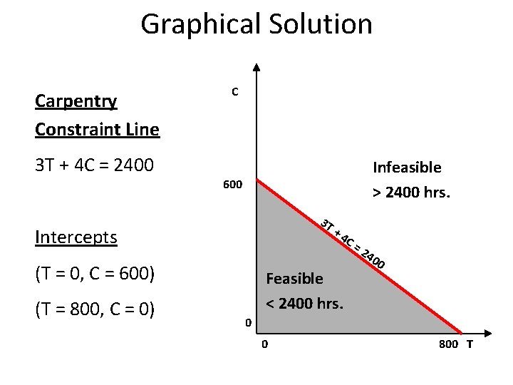
Graphical Solution Carpentry Constraint Line 3 T + 4 C = 2400 C Infeasible > 2400 hrs. 600 3 T Intercepts (T = 0, C = 600) (T = 800, C = 0) +4 Feasible < 2400 hrs. C= 24 00 0 0 800 T

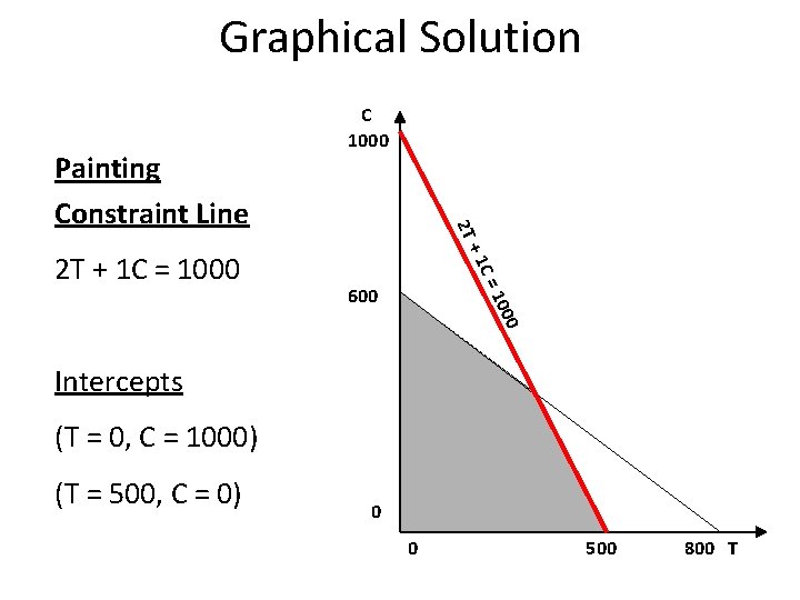
Graphical Solution C= +1 2 T + 1 C = 1000 2 T Painting Constraint Line C 1000 0 100 600 Intercepts (T = 0, C = 1000) (T = 500, C = 0) 0 0 500 800 T

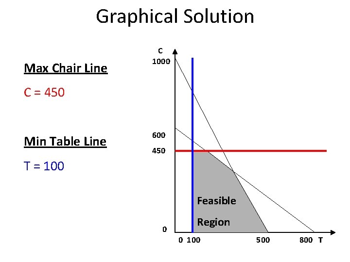
Graphical Solution Max Chair Line C 1000 C = 450 Min Table Line 600 450 T = 100 Feasible 0 Region 0 100 500 800 T

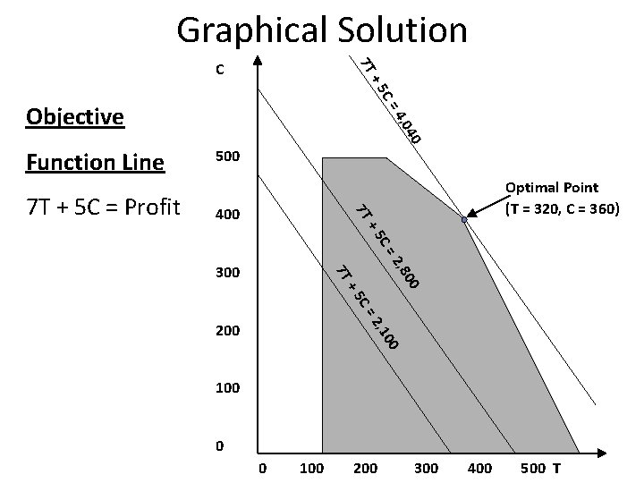
Graphical Solution 7 T C C= +5 4, 0 Objective 40 Function Line 400 Optimal Point (T = 320, C = 360) 7 T 7 T + 5 C = Profit 500 C= +5 2, 8 C= +5 00 7 T 300 2, 1 200 00 100 0 0 100 200 300 400 500 T

Graphical Solution

Special Situations in Linear Programming

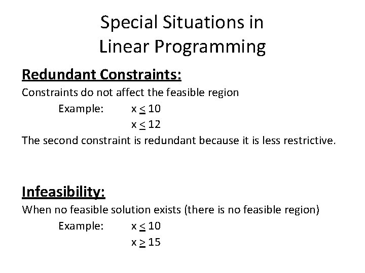
Special Situations in Linear Programming Redundant Constraints: Constraints do not affect the feasible region Example: x < 10 x < 12 The second constraint is redundant because it is less restrictive. Infeasibility: When no feasible solution exists (there is no feasible region) Example: x < 10 x > 15

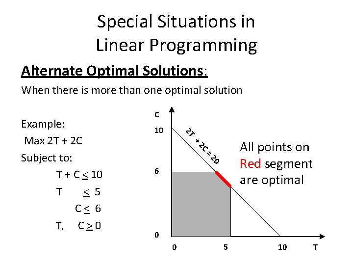
Special Situations in Linear Programming Alternate Optimal Solutions: When there is more than one optimal solution 10 2 T All points on Red segment are optimal C +2 =2 0 Example: Max 2 T + 2 C Subject to: T + C < 10 T < 5 C< 6 T, C > 0 C 6 0 0 5 10 T

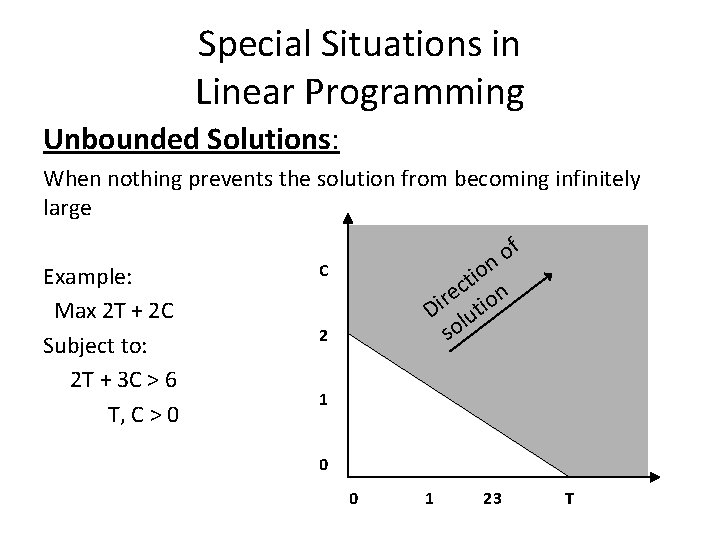
Special Situations in Linear Programming Unbounded Solutions: When nothing prevents the solution from becoming infinitely large Example: Max 2 T + 2 C Subject to: 2 T + 3 C > 6 T, C > 0 f o n o i t c ri e tion D lu so C 2 1 0 0 1 23 T

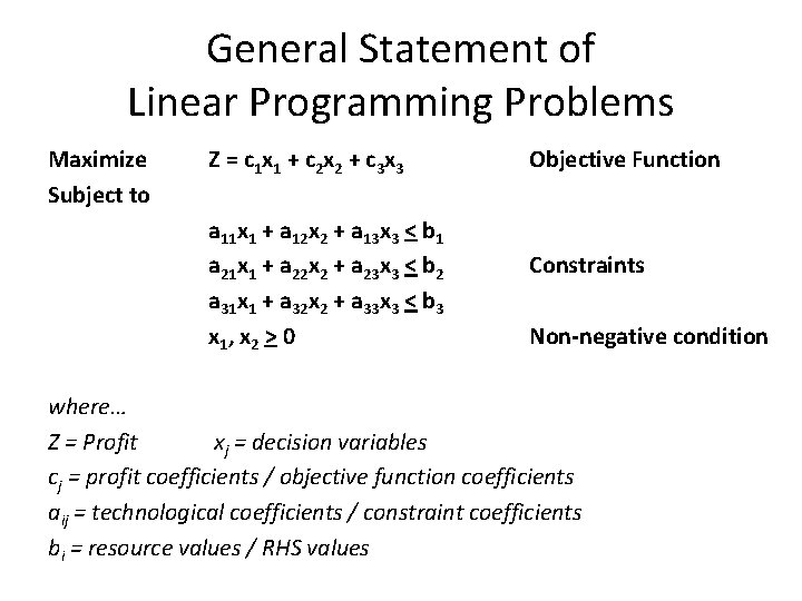
General Statement of Linear Programming Problems

General Statement of Linear Programming Problems Maximize Subject to Z = c 1 x 1 + c 2 x 2 + c 3 x 3 a 11 x 1 + a 12 x 2 + a 13 x 3 < b 1 a 21 x 1 + a 22 x 2 + a 23 x 3 < b 2 a 31 x 1 + a 32 x 2 + a 33 x 3 < b 3 x 1, x 2 > 0 Objective Function Constraints Non-negative condition where… Z = Profit xj = decision variables cj = profit coefficients / objective function coefficients aij = technological coefficients / constraint coefficients bi = resource values / RHS values