Lecture No 14 Management Course Engineering CHAPTER11 MATHEMATICAL

Lecture No. 14 Management Course: Engineering CHAPTER#11 MATHEMATICAL MODELS FOR ENGINEERING MANAGEMENT DECISION MAKING COURSE INSTRUCTOR : PROF. DR. SHAHAB KHUSHNOOD MED DEPARTMENT, U. E. T TAXILA

INTRODUCTION Mathematical Model is used to provide useful input factors in engineering management decision making. The models in this chapter basically fall into the following three areas. 1 - Cost-Capacity. 2 - Financial Investment Modeling. 3 - Equipment Repair.

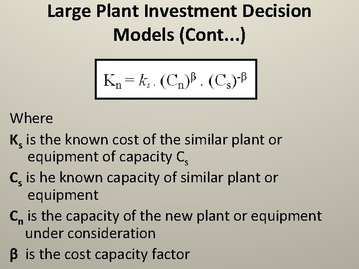
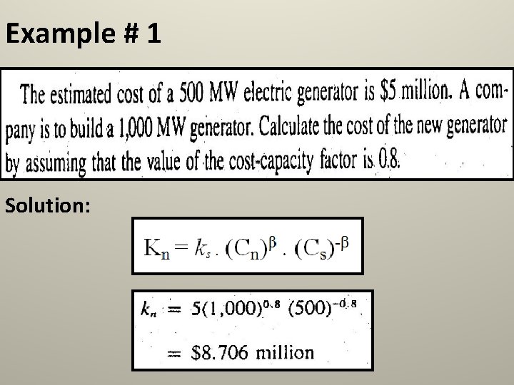
Large Plant Investment Decision Models Model 1: • This model is known as cost capacity model. • In this model it is assumed that for equipment or a plant under consideration, cost data on similar equipment or plant of different capacity is available. • Thus the cost of a new equipment or plant, Kn, under consideration may be calculated by utilizing the following equation

Large Plant Investment Decision Models (Cont. . . ) Where Ks is the known cost of the similar plant or equipment of capacity Cs Cs is he known capacity of similar plant or equipment Cn is the capacity of the new plant or equipment under consideration β is the cost capacity factor

Example # 1 Solution:

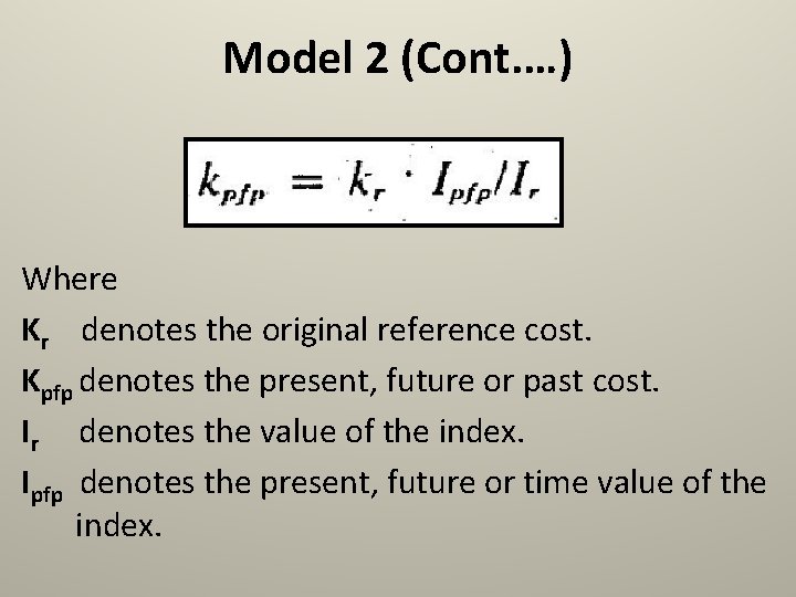
Large Plant Investment Decision Models (Cont. . . ) Model 2: • This model is known as the Cost Index. • This is used for comparison purposes. • A cost index for a specified period or time shows the cost at that time in relation to a given base year. • Thus the following formula is used to predict present, future or past cost.

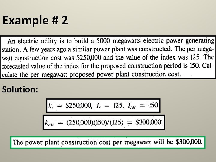
Model 2 (Cont. …) Where Kr denotes the original reference cost. Kpfp denotes the present, future or past cost. Ir denotes the value of the index. Ipfp denotes the present, future or time value of the index.

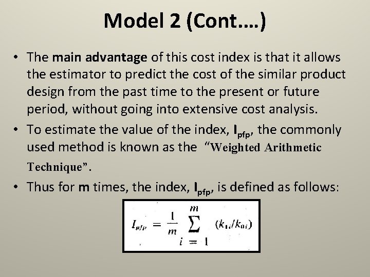
Model 2 (Cont. …) • The main advantage of this cost index is that it allows the estimator to predict the cost of the similar product design from the past time to the present or future period, without going into extensive cost analysis. • To estimate the value of the index, Ipfp, the commonly used method is known as the “Weighted Arithmetic Technique”. • Thus for m times, the index, Ipfp, is defined as follows:

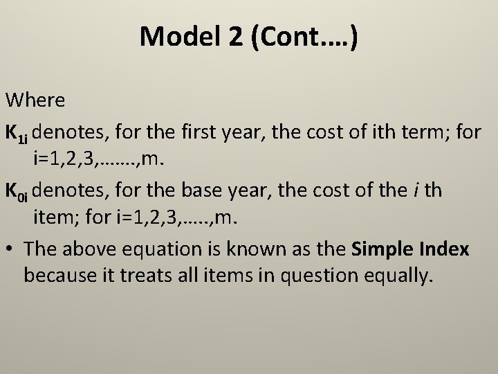
Model 2 (Cont. …) Where K 1 i denotes, for the first year, the cost of ith term; for i=1, 2, 3, ……. , m. K 0 i denotes, for the base year, the cost of the i th item; for i=1, 2, 3, …. . , m. • The above equation is known as the Simple Index because it treats all items in question equally.

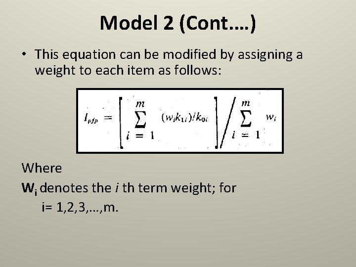
Model 2 (Cont. …) • This equation can be modified by assigning a weight to each item as follows: Where Wi denotes the i th term weight; for i= 1, 2, 3, …, m.

Example # 2 Solution:

Financial Investment Modeling • This is one mathematical model to determine the optimum area to be saved by a warehouse. • It is generally accepted that as the volume of goods in a warehouse increases, the warehousing costs per dollar’s worth of goods decreases. • In this model, it is assumed that a company has a number of warehouses. • If company increases the size of its warehouses, the number of warehouses required and good warehousing costs would be reduced in return.

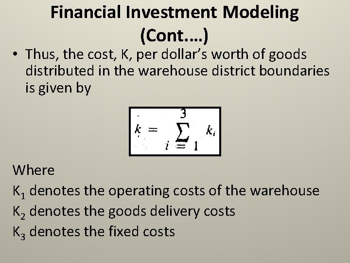
Financial Investment Modeling (Cont. …) • Thus, the cost, K, per dollar’s worth of goods distributed in the warehouse district boundaries is given by Where K 1 denotes the operating costs of the warehouse K 2 denotes the goods delivery costs K 3 denotes the fixed costs

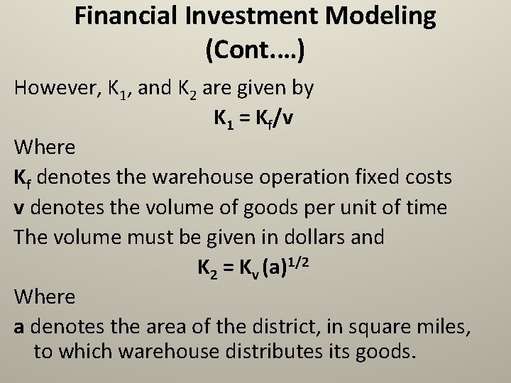
Financial Investment Modeling (Cont. …) However, K 1, and K 2 are given by K 1 = Kf/v Where Kf denotes the warehouse operation fixed costs v denotes the volume of goods per unit of time The volume must be given in dollars and K 2 = Kv (a)1/2 Where a denotes the area of the district, in square miles, to which warehouse distributes its goods.

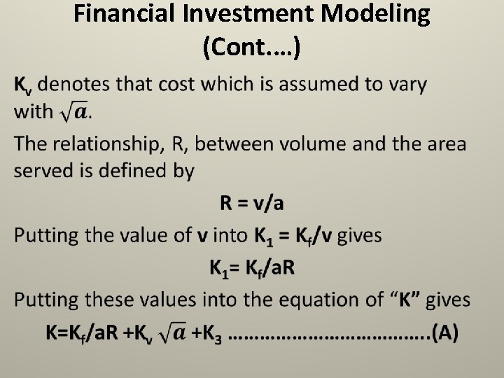
Financial Investment Modeling (Cont. …) •

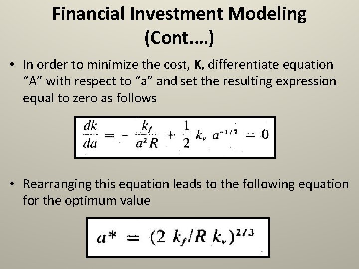
Financial Investment Modeling (Cont. …) • In order to minimize the cost, K, differentiate equation “A” with respect to “a” and set the resulting expression equal to zero as follows • Rearranging this equation leads to the following equation for the optimum value

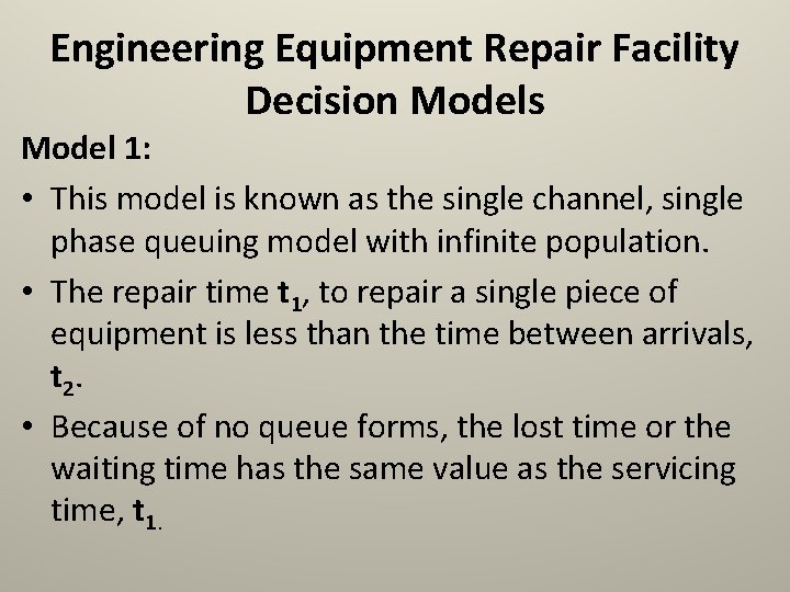
Engineering Equipment Repair Facility Decision Models Model 1: • This model is known as the single channel, single phase queuing model with infinite population. • The repair time t 1, to repair a single piece of equipment is less than the time between arrivals, t 2. • Because of no queue forms, the lost time or the waiting time has the same value as the servicing time, t 1.

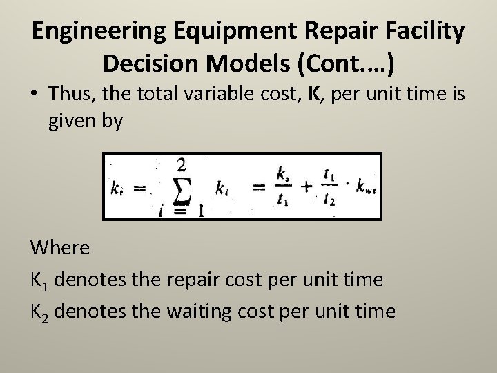
Engineering Equipment Repair Facility Decision Models (Cont. …) • Thus, the total variable cost, K, per unit time is given by Where K 1 denotes the repair cost per unit time K 2 denotes the waiting cost per unit time

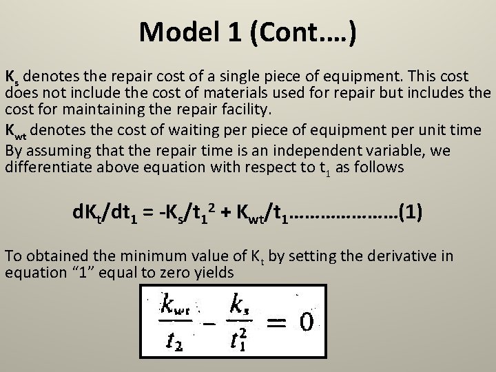
Model 1 (Cont. …) Ks denotes the repair cost of a single piece of equipment. This cost does not include the cost of materials used for repair but includes the cost for maintaining the repair facility. Kwt denotes the cost of waiting per piece of equipment per unit time By assuming that the repair time is an independent variable, we differentiate above equation with respect to t 1 as follows d. Kt/dt 1 = -Ks/t 12 + Kwt/t 1…………………(1) To obtained the minimum value of Kt by setting the derivative in equation “ 1” equal to zero yields

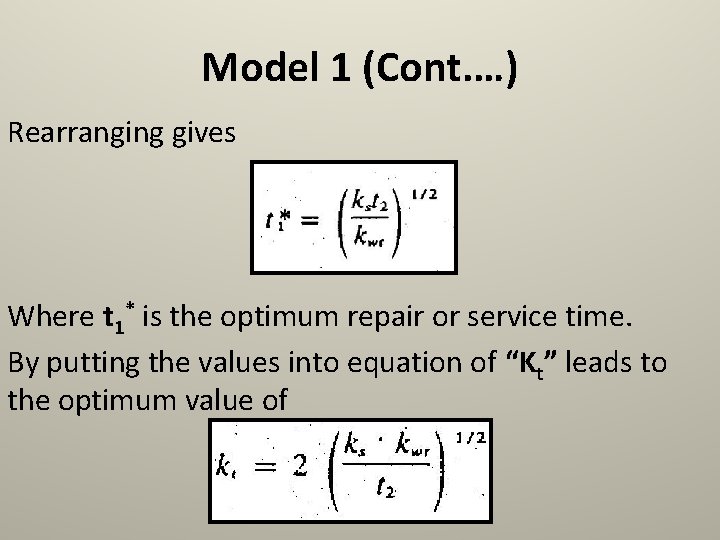
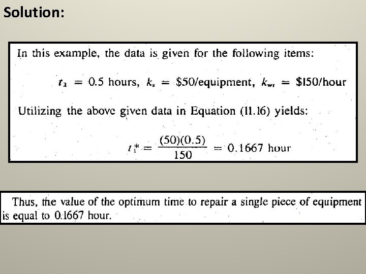
Model 1 (Cont. …) Rearranging gives Where t 1* is the optimum repair or service time. By putting the values into equation of “Kt” leads to the optimum value of

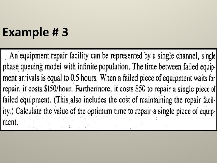
Example # 3

Solution:

Engineering Equipment Repair Facility Decision Models (Cont. …) Model 2: • This model is the result of further development on Model 1. • The only difference between this Model and Model 1 is that this one has “M” service or repair channels instead of only one.

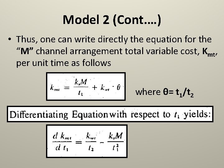
Model 2 (Cont. …) • Thus, one can write directly the equation for the “M” channel arrangement total variable cost, Kmt, per unit time as follows where θ= t 1/t 2

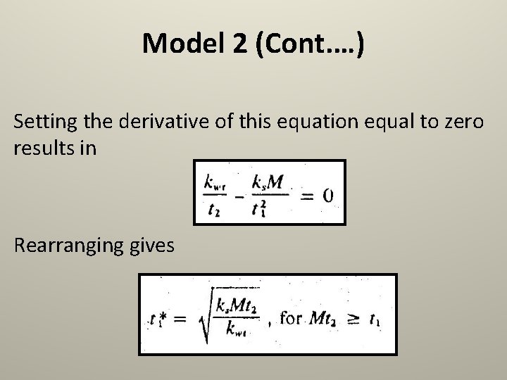
Model 2 (Cont. …) Setting the derivative of this equation equal to zero results in Rearranging gives

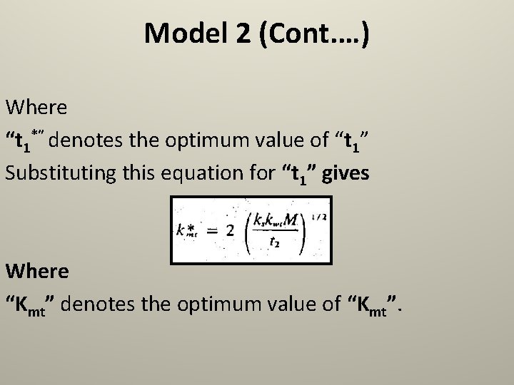
Model 2 (Cont. …) Where “t 1*” denotes the optimum value of “t 1” Substituting this equation for “t 1” gives Where “Kmt” denotes the optimum value of “Kmt”.

H T S K N A