Lecture 5 Optimization with equality constraints Constrained optimization

Lecture 5 – Optimization with equality constraints

Constrained optimization The idea of constrained optimisation is that the choice of one variable often affects the amount of another variable that can be used Eg if a firm employs more labour, this may affect the amount of capital it can afford to rent if it is restricted (constrained) by how much it can spend on inputs when a consumer maximizes utility (the ‘objective function’), x and y must be affordable – income provides the constraint. When a government sets expenditure levels it faces constraints set by its income from taxes Any optimal (eg profit maximising, cost minimising) quantities obtained when under a constraint may be different from the quantities that might be achieved if the agent were unconstrained 2

Binding and non-binding constraints A constraint is binding if at the optimum the constraint function holds with equality (sometimes called an equality constraint) giving a boundary solution somewhere on the constraint itself Otherwise the constraint is non-binding or slack (sometimes called an inequality constraint) If the constraint is binding we can use the Lagrangean technique 3

Often we can use our economic understanding to tell us if a constraint is binding – Example: a non-satiated consumer will always spend all her income so the budget constraint will be satisfied with equality But in general we do not know whether a constraint will be binding ( = , > or < ) In this case we use a technique which is related to the Lagrangean, but which is slightly more general called linear programming, or in the case of non-linear inequality constraints, non-linear programming or Kuhn-Tucker programming after its main inventors 4

Objectives and constraints - example A firm chooses output x to maximize a profit function π = -x 2 + 10 x - 6 Because of a staff shortage, it cannot produce an output higher than x = 4 What are the objective and constraint functions? The objective function: π = -x 2 + 10 x-6 The constraint: x ≤ 4 π x 4 5

Note that without the constraint the optimum is x = 5 So the constraint is binding (but a constraint of, say, x ≤ 6 would not be) – In general it is not always easy to see this π 4 5 x 6

Constrained optimization with two variables and one constraint •

y x

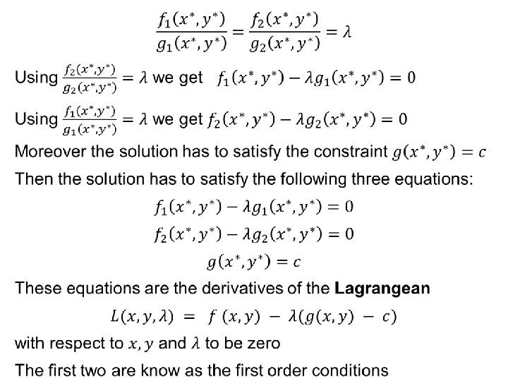
Procedure for the solution • 11

Interpretation of λ •

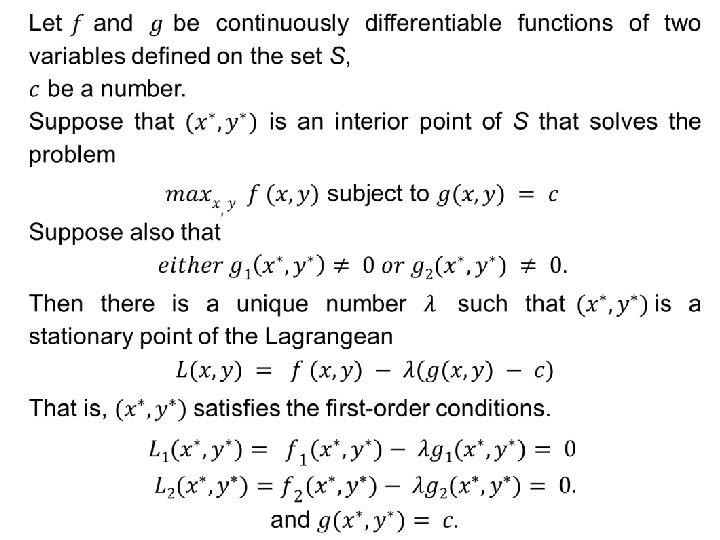
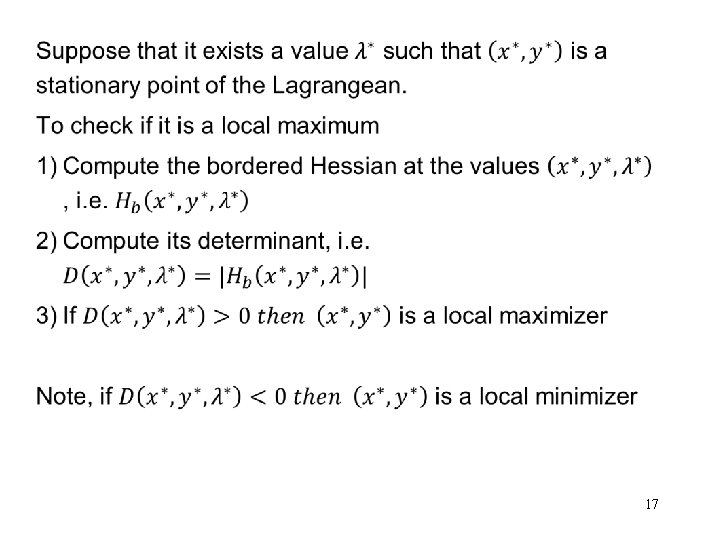
Conditions under which a stationary point is a local optimum •

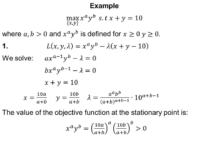
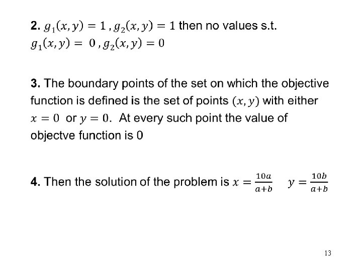
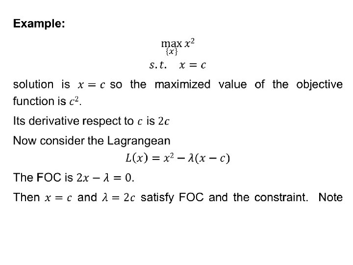
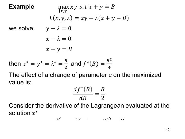
Example • 18

Conditions under which a stationary point is a global optimum • Suppose that f and g are continuously differentiable functions defined on an open convex subset S of twodimensional space and • suppose that there exists a number λ* such that (x*, y*) is an interior point of S that is a stationary point of the Lagrangean L(x, y) = f (x, y) − λ*(g(x, y) − c). • Suppose further that g(x*, y*) = c. • Then if L is concave then (x*, y*) solves the problem maxx, y f (x, y) subject to g(x, y) = c

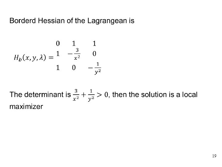
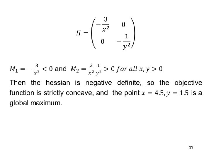
Example • 21

Optimization with equality constraints: n variables, m constraints Let f and g 1, . . . , gm be continuously differentiable functions of n variables defined on the set S, let cj for j = 1, . . . , m be numbers, and suppose that x* is an interior point of S that solves the problem: maxx f (x) subject to gj(x) = cj for j = 1, . . . , m Suppose also that (∂gj/∂xi)(x*) � 0 for all i

Then there are unique numbers λ 1, . . . , λm such that x* is a stationary point of the Lagrangean function L defined by L(x) = f (x) − ∑j=1 mλj(gj(x) − cj). That is, x* satisfies the first-order conditions: L'i(x*) = f i'(x*) − ∑j=1 mλj(∂gj/∂xi)(x*) = 0 for i = 1, . . . , n. In addition, gj(x*) = cj for j = 1, . . . , m.

Conditions under which necessary conditions are sufficient Suppose that f and gj for j = 1, . . . , m are continuously differentiable functions defined on an open convex subset S of n-dimensional space and let x* ∈ S be an interior stationary point of the Lagrangean: L(x) = f (x) − ∑j=1 mλ*j(gj(x) − cj). Suppose further that gj(x*) = cj for j = 1, . . . , m. Then if L is concave then x* solves the constrained maximization problem

Interpretation of λ Consider the problem maxx f (x) subject to gj(x) = cj for j = 1, . . . , m, Let x*(c) be the solution of this problem, where c is the vector (c 1, . . . , cm) and let f *(c) = f (x*(c)). Then we have f *j'(c) = λj(c) for j = 1, . . . , m, where λj is the value of the Lagrange multiplier on the jth constraint at the solution of the problem.

Interpretation of λ The value of the Lagrange multiplier on the jth constraint at the solution of the problem is equal to the rate of change in the maximal value of the objective function as the jth constraint is relaxed. If the jth constraint arises because of a limit on the amount of some resource, then we refer to λj(c) as the shadow price of the jth resource.

Quasi-concave functions f(x″) = f(λx + (1 -λ)x‘ ) ≥ min(f(x), f(x’) ) quasi concave f(x″) = f(λx + (1 -λ)x‘ ) > min(f(x), f(x’) ) strictly quasi concave Note these conditions hold even if f(x)=f(x’) A concave function is also quasi-concave, but the opposite is not true If f(x) > f(x’) and f(λx + (1 -λ)x‘ ) > f(x’) the function is explicitly quasi concave 28

f(x″) = f(λx + (1 -λ)x’ ) ≤ max(f(x), f(x’) ) Note that a convex function is also quasi-convex The bottom left picture shows that the opposite is not true y y y 29

The importance of concavity and quasi-concavity • 30

Convex sets. A convex set, X, is such that for any two elements of the set, x and x’ any convex combination of them is also a member of the set. x x' More formally, X is convex if for all x and x’ ε X, and 0 ≤λ≤ 1, x″ = λx + (1 -λ)x‘ ε X. Sometimes X is described as strictly convex if for any 0 < λ <1, x″ is in the interior of X (i. e. not on the edges) e. g. convex but not strictly convex 31

Convex sets. If, for any two points in the set S, the line segment connecting these two points lie entirely in S, then S is a convex set. U x 2 p 1 x 1+p 2 x 2 ≤ m x 1 U(x)≥ U x 32 1

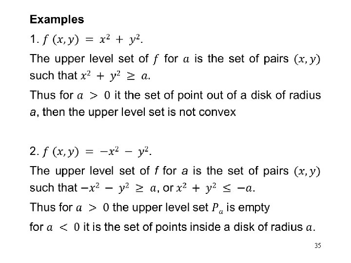
Non-Convex sets. U x 2 U(x)≤ U 33 x 1

A different definition of quasi concavity • 34

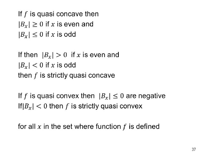
Checking quasi concavity • 36

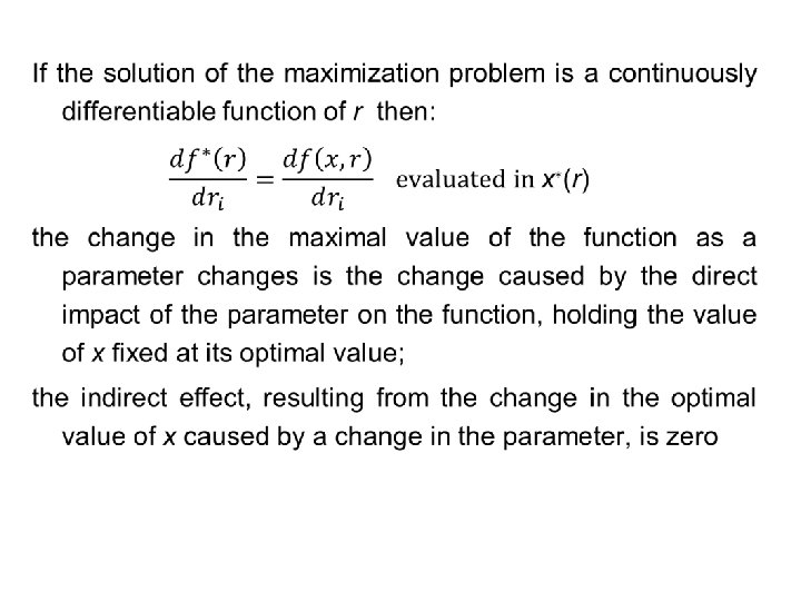
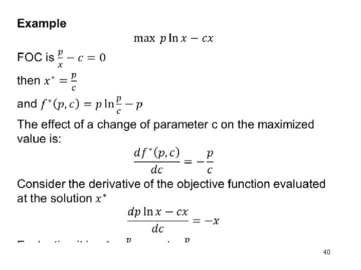
Envelope theorem: unconstrained problem •

Envelope theorem: constrained problems •