Ch 12 Optimization with Equality Constraints 12 1

Ch. 12 Optimization with Equality Constraints • • • 12. 1 12. 2 12. 3 12. 4 12. 5 Demand • 12. 6 • 12. 7 • 12. 8 Effects of a Constraint Finding the Stationary Values Second-Order Conditions Quasi-concavity and Quasi-convexity Utility Maximization and Consumer Homogeneous Functions Least-Cost Combination of Inputs Some concluding remarks 1

2

3

4

5

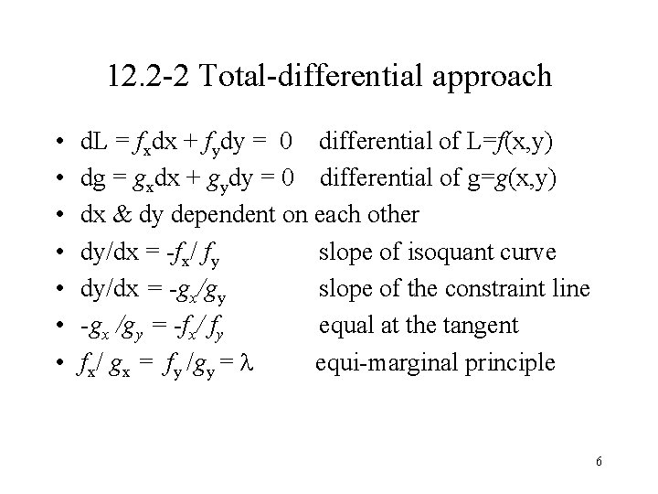
12. 2 -2 Total-differential approach • • d. L = fxdx + fydy = 0 differential of L=f(x, y) dg = gxdx + gydy = 0 differential of g=g(x, y) dx & dy dependent on each other dy/dx = -fx/ fy slope of isoquant curve dy/dx = -gx/gy slope of the constraint line -gx /gy = -fx/ fy equal at the tangent fx/ gx = fy /gy = equi-marginal principle 6

7

8

9

10

11

12

13

12. 2 Finding the Stationary Values • 12. 2 -1 Lagrange-multiplier method • 12. 2 -2 Total-differential approach • 12. 2 -3 An interpretation of the Lagrange multiplier • 12. 2 -4 n-variable and multi-constraint case 14

12. 2 -1 Lagrange-multiplier method 15

12. 2 -2 Total-differential approach • • d. L = fxdx + fydy = 0 differential of L=f(x, y) dg = gxdx + gydy = 0 differential of g=g(x, y) dx & dy dependent on each other dy/dx = -fx/ fy slope of isoquant curve dy/dx = -gx/gy slope of the constraint line -gx /gy = -fx/ fy equal at the tangent fx/ gx = fy /gy = equi-marginal principle 16

17

18

12. 3 • • • Second-Order Conditions 12. 3 -1 Second-order total differential 12. 3 -2 Second-order conditions 12. 3 -3 The bordered Hessian 12. 3 -4 n-variable case 12. 3 -5 Multi-constraint case 19

11. 4 n-variable soc principal minors test for unconstrained max or min 20

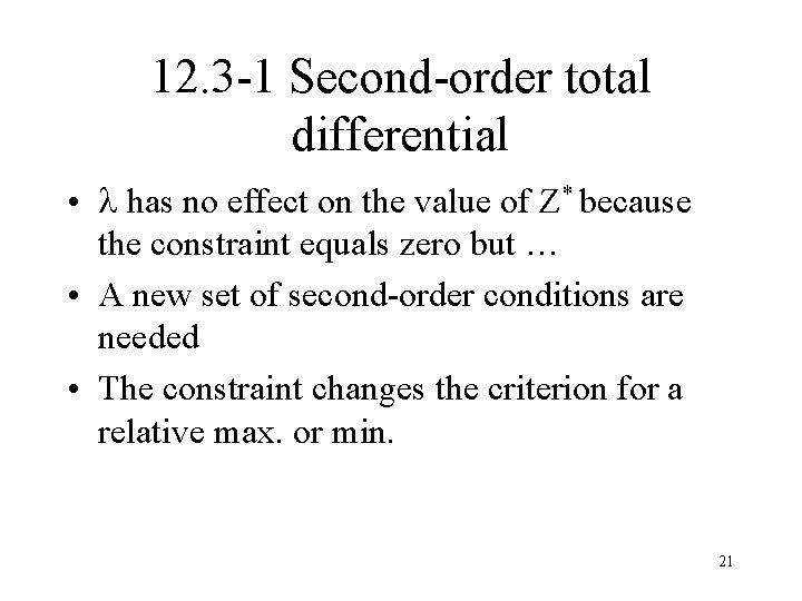
12. 3 -1 Second-order total differential • has no effect on the value of Z* because the constraint equals zero but … • A new set of second-order conditions are needed • The constraint changes the criterion for a relative max. or min. 21

12. 3 -1 Second-order total differential 22

12. 3 -1 Second-order total differential 23

24

25

26

12. 4 Quasi-concavity and Quasi-convexity • • 12. 4 -1 Geometric characterization 12. 4 -2 Algebraic definition 12. 4 -3 Differentiable functions 12. 4 -4 A further look at the bordered Hessian • 12. 4 -5 Absolute vs. relative extrema 27

12. 5 Utility Maximization and Consumer Demand • • 12. 5 -1 First-order condition 12. 5 -2 Second-order condition 12. 5 -3 Comparative-static analysis 12. 5 -4 Proportionate changes in prices and income 28

29

30

31

32

33

34

35

36

37

38

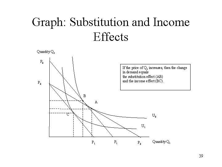
Graph: Substitution and Income Effects Quantity Q 2 P 0 If the price of Q 1 increases, then the change in demand equals the substitution effect (AB) and the income effect (BC). P 0 B A C U 0 U 1 P 1 P 0 Quantity Q 1 39

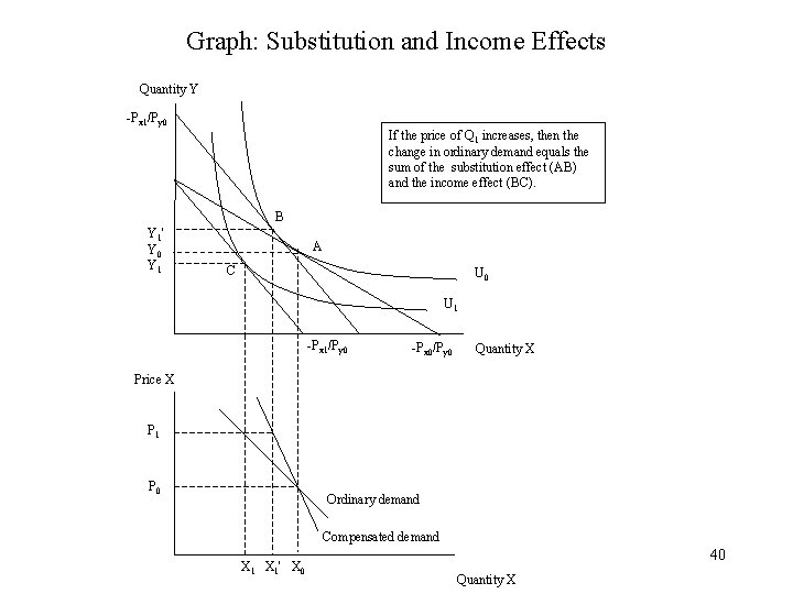
Graph: Substitution and Income Effects Quantity Y -Px 1/Py 0 If the price of Q 1 increases, then the change in ordinary demand equals the sum of the substitution effect (AB) and the income effect (BC). B Y 1' Y 0 Y 1 A C U 0 U 1 -Px 1/Py 0 -Px 0/Py 0 Quantity X Price X P 1 P 0 Ordinary demand Compensated demand X 1' X 0 40 Quantity X

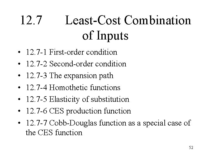
12. 7 • • Least-Cost Combination of Inputs 12. 7 -1 First-order condition 12. 7 -2 Second-order condition 12. 7 -3 The expansion path 12. 7 -4 Homothetic functions 12. 7 -5 Elasticity of substitution 12. 7 -6 CES production function 12. 7 -7 Cobb-Douglas function as a special case of the CES function 52

53

54

55

56

57

12. 7 -6 CES production function 64

12. 7 -6 CES production function 65

12. 7 -6 CES production function 66

12. 7 -6 CES production function 67

12. 7 -6 CES production function 68

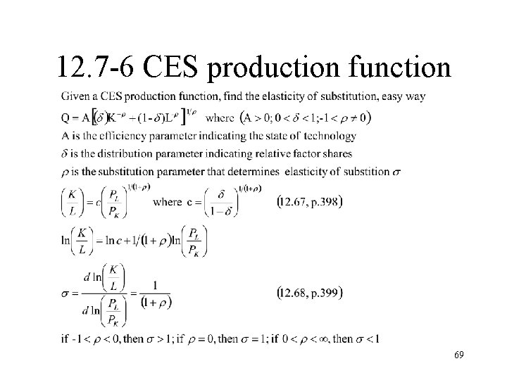
12. 7 -6 CES production function 69

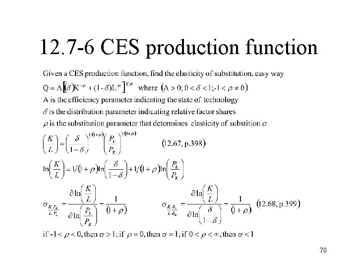
12. 7 -6 CES production function 70

12. 7 -6 CES production function 71