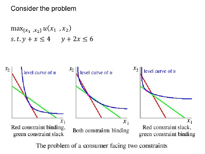
Optimization with inequality constraints Optimization with inequality constraints

Optimization with inequality constraints

Optimization with inequality constraints: the Kuhn-Tucker (KT) conditions •

When KT conditions are necessary • 5

• Example: KT are not necessary conditions for a max 6

• 0. 9 0. 7 0. 5 y C 1 1. 4 1. 6 0. 3 0. 1 0 0. 2 0. 4 0. 6 0. 8 1 1. 2 1. 8 2 -0. 1 -0. 3 -0. 5 7

the sufficiency of the Kuhn-Tucker conditions (1) • 9

the sufficiency of the Kuhn-Tucker conditions (2) • 10

Necessity and sufficiency of KT conditions A) The KT conditions are both necessary and sufficient – if the objective function is concave and – either each constraint is linear – or each constraint function is convex and some vector of the variables satisfies all constraints strictly.

Necessity and sufficiency of KT conditions B) Suppose that - the objective function is twice differentiable and quasiconcave and - every constraint is linear. Then - If x* solves the problem then there exists a unique vector λ such that (x*, λ) satisfies the Kuhn-Tucker conditions, and - if (x*, λ) satisfies the Kuhn-Tucker conditions and f 'i(x*) ≠ 0 for i = 1, . . . , n then x* solves the problem.

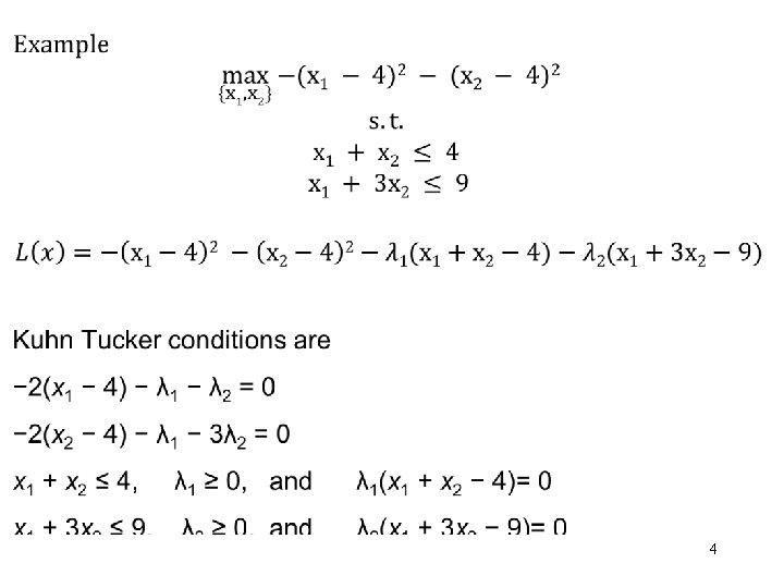
Example • 13

Kuhn Tucker conditions are − 2(x 1 − 4) − λ 1 − λ 2 = 0 − 2(x 2 − 4) − λ 1 − 3λ 2 = 0 x 1 + x 2 ≤ 4, λ 1 ≥ 0, and λ 1(x 1 + x 2 − 4)= 0 x 1 + 3 x 2 ≤ 9, λ 2 ≥ 0, and λ 2(x 1 + 3 x 2 − 9)= 0 To solve this system of condition we have to consider all possibilities about the values of lambdas We have to consider the following 4 cases: 1) λ 1 = λ 2 = 0 2) λ 1 >0 λ 2 = 0 3) λ 1 =0 λ 2 > 0 4) λ 1 >0 λ 2 > 0 14

Kuhn Tucker conditions are − 2(x 1 − 4) − λ 1 − λ 2 = 0 − 2(x 2 − 4) − λ 1 − 3λ 2 = 0 x 1 + x 2 ≤ 4, λ 1 ≥ 0, and λ 1(x 1 + x 2 − 4)= 0 x 1 + 3 x 2 ≤ 9, λ 2 ≥ 0, and λ 2(x 1 + 3 x 2 − 9)= 0 Case 1: λ 1 = λ 2 = 0 KT conditions are − 2(x 1 − 4) = 0 − 2(x 2 − 4) = 0 x 1 + x 2 ≤ 4, x 1 + 3 x 2 ≤ 9 Then x 1 = 4 and x 2 =4 It not a solution because the last two inequalities are not satisfied 15

Kuhn Tucker conditions are − 2(x 1 − 4) − λ 1 − λ 2 = 0 − 2(x 2 − 4) − λ 1 − 3λ 2 = 0 x 1 + x 2 ≤ 4, λ 1 ≥ 0, and λ 1(x 1 + x 2 − 4)= 0 x 1 + 3 x 2 ≤ 9, λ 2 ≥ 0, and λ 2(x 1 + 3 x 2 − 9)= 0 Case 2: λ 1 >0 λ 2 = 0 KT conditions are − 2(x 1 − 4) − λ 1 = 0 − 2(x 2 − 4) − λ 1 = 0 x 1 + x 2 − 4= 0 x 1 + 3 x 2 ≤ 9, From the first 2 equations x 1 = x 2 Using the third equation we get x 1 = x 2 =2 and λ 1=4 It is a solution because the last inequality is satisfied 16

Kuhn Tucker conditions are − 2(x 1 − 4) − λ 1 − λ 2 = 0 − 2(x 2 − 4) − λ 1 − 3λ 2 = 0 x 1 + x 2 ≤ 4, λ 1 ≥ 0, and λ 1(x 1 + x 2 − 4)= 0 x 1 + 3 x 2 ≤ 9, λ 2 ≥ 0, and λ 2(x 1 + 3 x 2 − 9)= 0 Case 3: λ 1 =0 λ 2 > 0 KT conditions are − 2(x 1 − 4) − λ 2 = 0 − 2(x 2 − 4) − 3λ 2 = 0 x 1 + x 2 ≤ 4 x 1 + 3 x 2 − 9= 0 From the first 2 equations x 2=3 x 1 -8 Using the last equation we get x 1 = 3. 3 17 It is not a solution because it does not satisfy the inequality

Kuhn Tucker conditions are − 2(x 1 − 4) − λ 1 − λ 2 = 0 − 2(x 2 − 4) − λ 1 − 3λ 2 = 0 x 1 + x 2 ≤ 4, λ 1 ≥ 0, and λ 1(x 1 + x 2 − 4)= 0 x 1 + 3 x 2 ≤ 9, λ 2 ≥ 0, and λ 2(x 1 + 3 x 2 − 9)= 0 Case 4: λ 1 >0 λ 2 > 0 KT conditions are − 2(x 1 − 4) − λ 1 − λ 2 = 0 − 2(x 2 − 4) − λ 1 − 3λ 2 = 0 x 1 + x 2 − 4= 0 x 1 + 3 x 2 = 0 18

KT conditions are − 2(x 1 − 4) − λ 1 − λ 2 = 0 − 2(x 2 − 4) − λ 1 − 3λ 2 = 0 x 1 + x 2 − 4= 0 x 1 + 3 x 2 = 0 Using the last two equation we get x 1=1. 5 and x 2 =2. 5 Replacing in the first two equation we get the values of lambdas λ 1 =6 λ 2 = - 1 This is not a solution because it violates the condition λ 2 ≥ 0. 19

Solution is x 1 = x 2 =2 and λ 1=4 20

Optimization with inequality constraints: non negativity constraints •

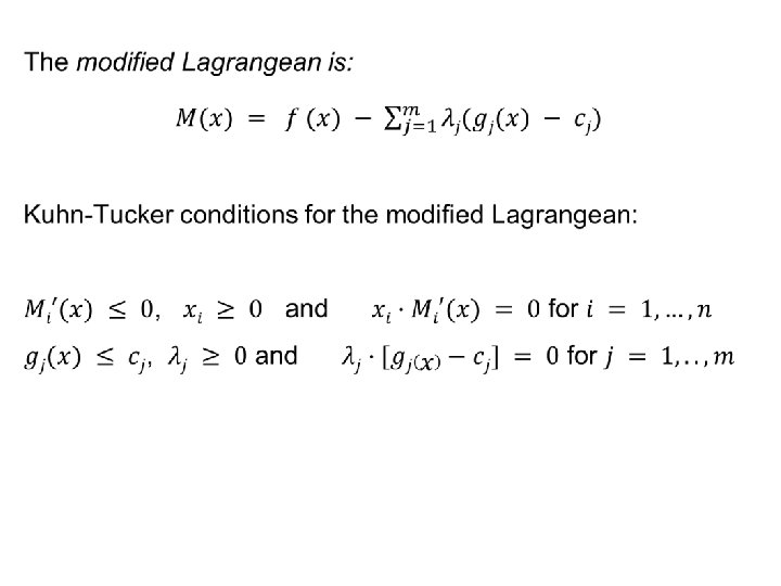
Specifically, if we define the function gm+i for i = 1, . . . , n by gm+i(x) = −xi and let cm+i = 0 for i = 1, . . . , n, then we may write the problem as maxx f (x) subject to gj(x) ≤ cj for j = 1, . . . , m+n and solve it using the Kuhn-Tucker conditions

Optimization with inequality constraints: non negativity constraints •

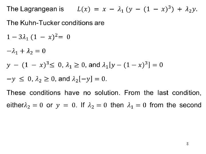
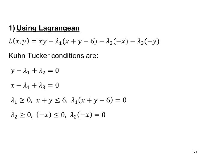
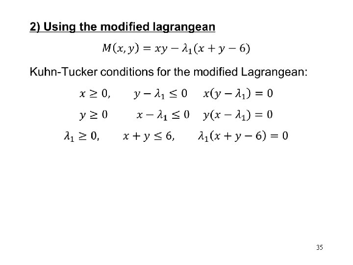
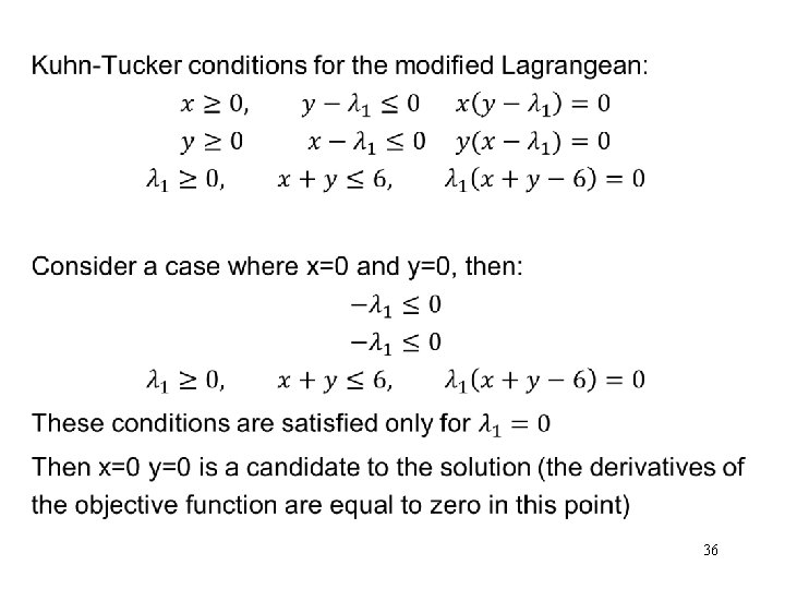
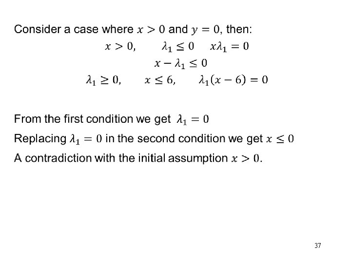
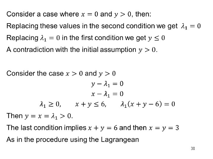
in any problem for which the original Kuhn-Tucker conditions may be used, we may alternatively use the conditions for the modified Lagrangean. For most problems in which the variables are constrained to be nonnegative, the Kuhn-Tucker conditions for the modified Lagrangean are easier than the conditions for the original Lagrangean Example. Consider the problem maxx, y xy subject to x + y ≤ 6, x ≥ 0, and y ≥ 0

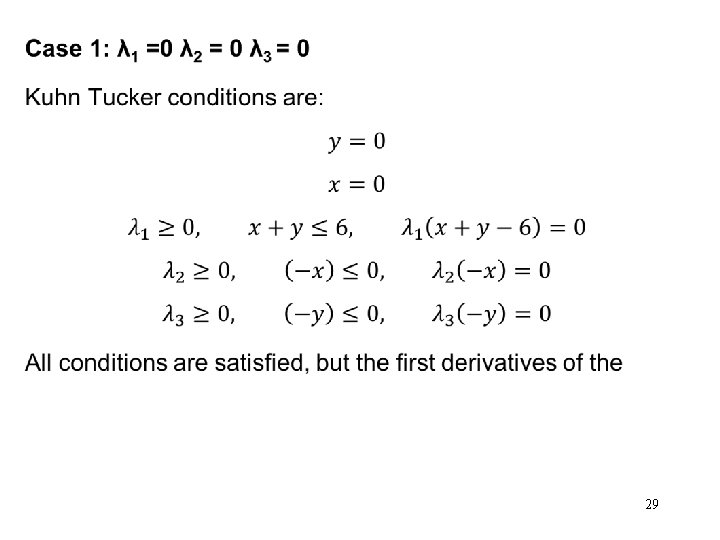
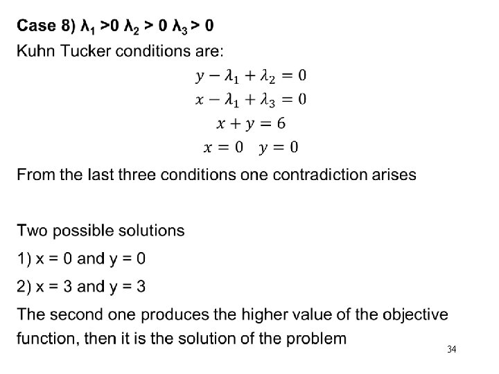
Function xy is twice-differentiable and quasiconcave and the constraint functions are linear, so the Kuhn-Tucker conditions are necessary and if ((x*, y*), λ*) satisfies these conditions and no partial derivative of the objective function at (x*, y*) is zero then (x*, y*) solves the problem. Solutions of the Kuhn-Tucker conditions at which all derivatives of the objective function are zero may or may not be solutions of the problem We try to solve it 1) using the lagrangean 2) Using the modified lagrangean

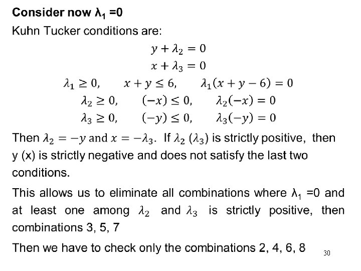
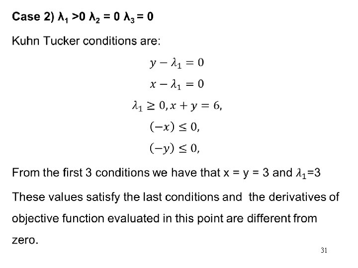
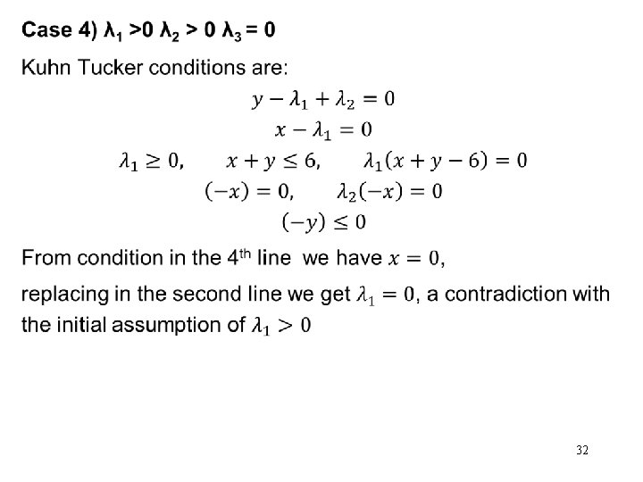
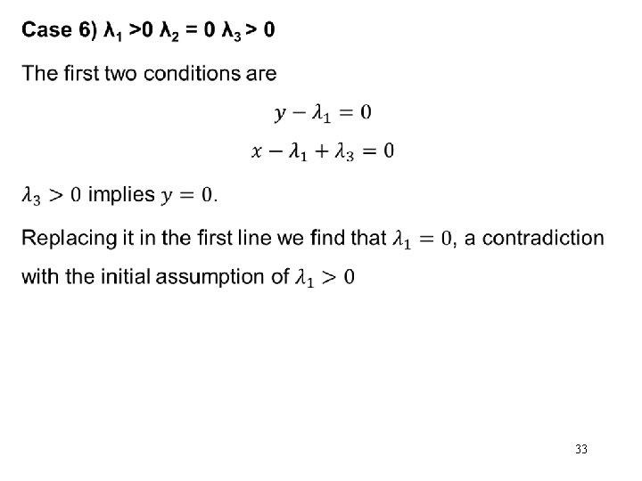
We have to consider the following 8 cases: 1) λ 1 =0 λ 2 = 0 λ 3 = 0 2) λ 1 >0 λ 2 = 0 λ 3 = 0 3) λ 1 =0 λ 2 > 0 λ 3 = 0 4) λ 1 >0 λ 2 > 0 λ 3 = 0 5) λ 1 =0 λ 2 = 0 λ 3 > 0 6) λ 1 >0 λ 2 = 0 λ 3 > 0 7) λ 1 =0 λ 2 > 0 λ 3 > 0 8) λ 1 >0 λ 2 > 0 λ 3 > 0 28

• http: //www. economics. utoronto. ca/osborne/Math. Tutorial/OSMF. HTM 39