Lecture 3 Introduction to Monte Carlo Markov chain

Lecture 3 Introduction to Monte Carlo Markov chain (MCMC) methods

Lecture Contents • • • How does Win. BUGS fit a regression? Gibbs Sampling Convergence and burnin How many iterations? Logistic regression example

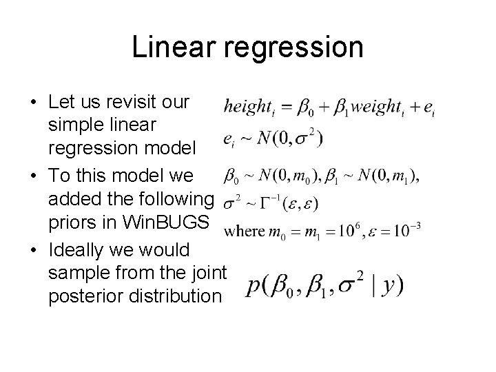
Linear regression • Let us revisit our simple linear regression model • To this model we added the following priors in Win. BUGS • Ideally we would sample from the joint posterior distribution

Linear Regression ctd. • In this case we can sample from the joint posterior as described in the last lecture • However this is not the case for all models and so we will now describe other simulation-based methods that can be used. • These methods come from a family of methods called Markov chain Monte Carlo (MCMC) methods and here we will focus on a method called Gibbs Sampling.

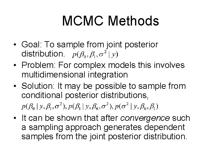
MCMC Methods • Goal: To sample from joint posterior distribution. • Problem: For complex models this involves multidimensional integration • Solution: It may be possible to sample from conditional posterior distributions, • It can be shown that after convergence such a sampling approach generates dependent samples from the joint posterior distribution.

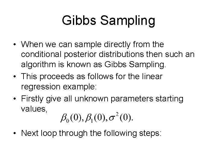
Gibbs Sampling • When we can sample directly from the conditional posterior distributions then such an algorithm is known as Gibbs Sampling. • This proceeds as follows for the linear regression example: • Firstly give all unknown parameters starting values, • Next loop through the following steps:

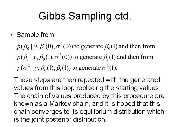
Gibbs Sampling ctd. • Sample from These steps are then repeated with the generated values from this loop replacing the starting values. The chain of values produced by this procedure are known as a Markov chain, and it is hoped that this chain converges to its equilibrium distribution which is the joint posterior distribution.

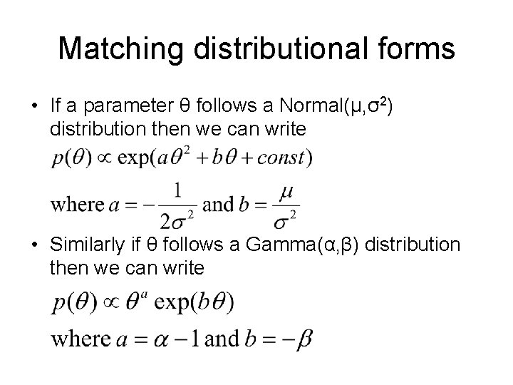
Calculating the conditional distributions • In order for the algorithm to work we need to sample from the conditional posterior distributions. • If these distributions have standard forms then it is easy to draw random samples from them. • Mathematically we write down the full posterior and assume all parameters are constants apart from the parameter of interest. • We then try to match the resulting formulae to a standard distribution.

Matching distributional forms • If a parameter θ follows a Normal(μ, σ2) distribution then we can write • Similarly if θ follows a Gamma(α, β) distribution then we can write

Step 1: β 0

Step 2: β 1

Step 3: 1/σ2

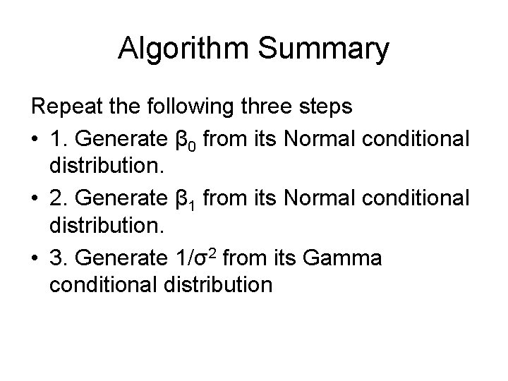
Algorithm Summary Repeat the following three steps • 1. Generate β 0 from its Normal conditional distribution. • 2. Generate β 1 from its Normal conditional distribution. • 3. Generate 1/σ2 from its Gamma conditional distribution

Convergence and burn-in Two questions that immediately spring to mind are: 1. We start from arbitrary starting values so when can we safely say that our samples are from the correct distribution? 2. After this point how long should we run the chain for and store values?

Checking Convergence This is the researchers responsibility! • Convergence is to a target distribution (the required posterior), not to a single value as in ML methods. • Once convergence has been reached, samples should look like a random scatter about a stable mean value.

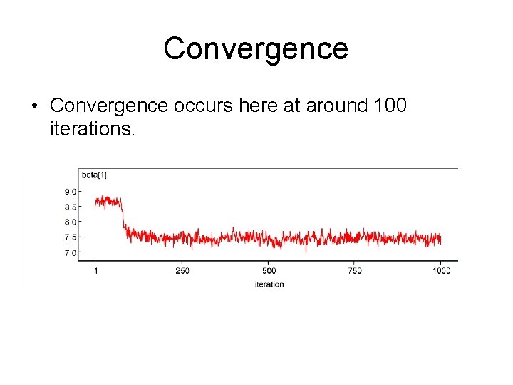
Convergence • Convergence occurs here at around 100 iterations.

Checking convergence 2 • One approach (in Win. BUGS) is to run many long chains with widely differing starting values. • Win. BUGS also has the Brooks-Gelman-Rubin diagnostic which is based on the ratio of between-within chain variances (ANOVA). This diagnostic should converge to 1. 0 on convergence. • MLwi. N has other diagnostics that we will cover on Wednesday.

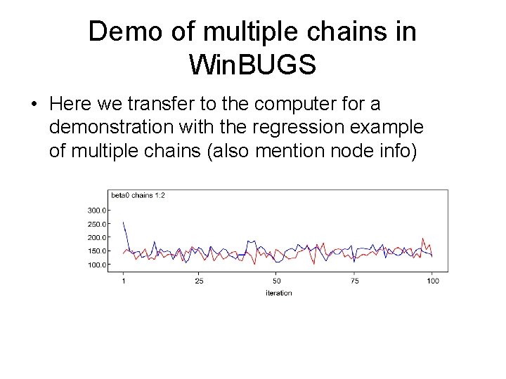
Demo of multiple chains in Win. BUGS • Here we transfer to the computer for a demonstration with the regression example of multiple chains (also mention node info)

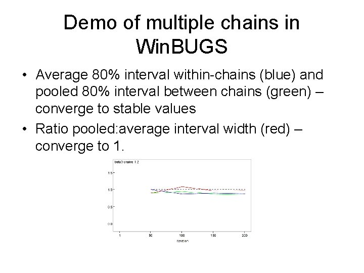
Demo of multiple chains in Win. BUGS • Average 80% interval within-chains (blue) and pooled 80% interval between chains (green) – converge to stable values • Ratio pooled: average interval width (red) – converge to 1.

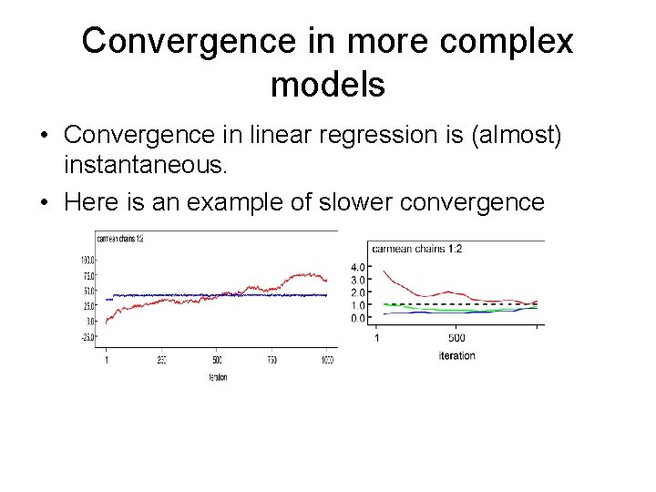
Convergence in more complex models • Convergence in linear regression is (almost) instantaneous. • Here is an example of slower convergence

How many iterations after convergence? • After convergence, further iterations are needed to obtain samples for posterior inference. • More iterations = more accurate posterior estimates. • MCMC chains are dependent samples and so the dependence or autocorrelation in the chain will influence how many iterations we need. • Accuracy of the posterior estimates can be assessed by the Monte Carlo standard error (MCSE) for each parameter. • Methods for calculating MCSE are given in later lectures.

Inference using posterior samples from MCMC runs • A powerful feature of MCMC and the Bayesian approach is that all inference is based on the joint posterior distribution. • We can therefore address a wide range of substantive questions by appropriate summaries of the posterior. • Typically report either the mean or median of the posterior samples for each parameter of interest as a point estimate • 2. 5% and 97. 5% percentiles of the posterior sample for each parameter give a 95% posterior credible interval (interval within which the parameter lies with probability 0. 95)

Derived Quantities • Once we have a sample from the posterior we can answer lots of questions simply by investigating this sample. Examples: What is the probability that θ>0? What is the probability that θ 1> θ 2? What is a 95% interval for θ 1/(θ 1+ θ 2)? See later for examples of these sorts of derived quantities.

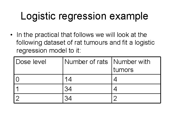
Logistic regression example • In the practical that follows we will look at the following dataset of rat tumours and fit a logistic regression model to it: Dose level 0 1 2 Number of rats Number with tumors 14 4 34 2

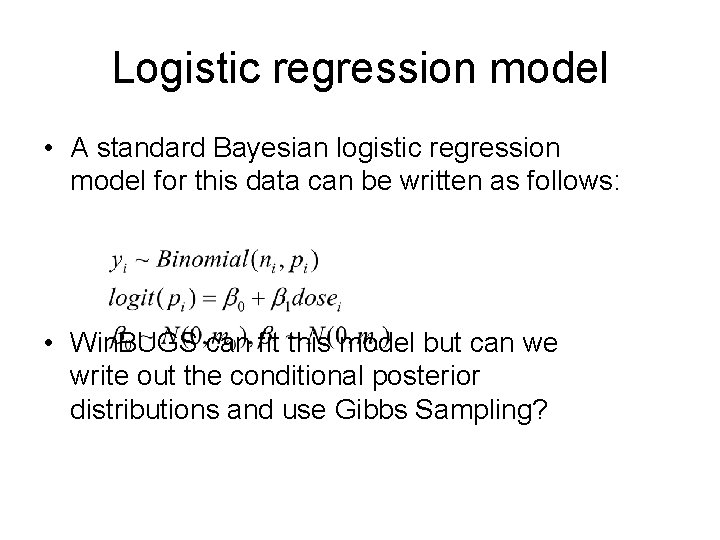
Logistic regression model • A standard Bayesian logistic regression model for this data can be written as follows: • Win. BUGS can fit this model but can we write out the conditional posterior distributions and use Gibbs Sampling?

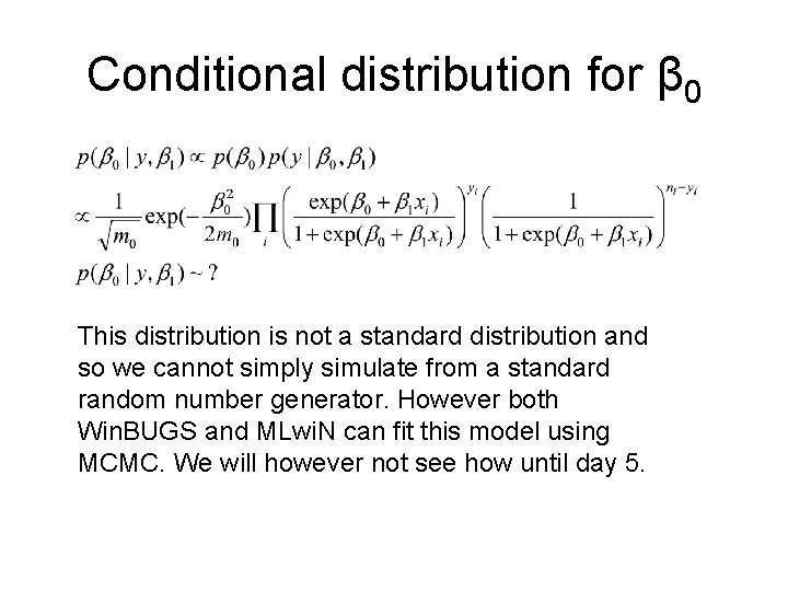
Conditional distribution for β 0 This distribution is not a standard distribution and so we cannot simply simulate from a standard random number generator. However both Win. BUGS and MLwi. N can fit this model using MCMC. We will however not see how until day 5.

Hints for the next practical • In the next practical you will be creating Win. BUGS code for a logistic regression model. • In this practical you get less help and so I would suggest that looking at the Seeds example in the Win. BUGS examples may help. The seeds example is more complicated than what you require but will be helpful for showing the necessary Win. BUGS statements.