Lecture 12 Agenda Longitudinal study design and longitudinal

Lecture 12

Agenda • Longitudinal study design and longitudinal data • Within subject correlation • Summarizing Longitudinal Data • Basic Technique – Analysis of Response Profiles

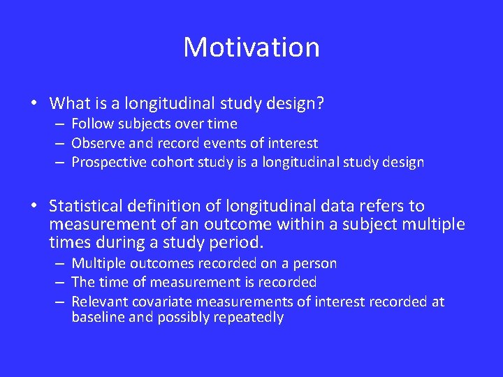
Motivation • What is a longitudinal study design? – Follow subjects over time – Observe and record events of interest – Prospective cohort study is a longitudinal study design • Statistical definition of longitudinal data refers to measurement of an outcome within a subject multiple times during a study period. – Multiple outcomes recorded on a person – The time of measurement is recorded – Relevant covariate measurements of interest recorded at baseline and possibly repeatedly

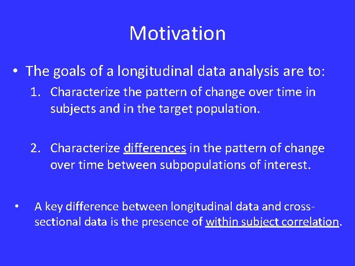
Motivation • The goals of a longitudinal data analysis are to: 1. Characterize the pattern of change over time in subjects and in the target population. 2. Characterize differences in the pattern of change over time between subpopulations of interest. • A key difference between longitudinal data and crosssectional data is the presence of within subject correlation.

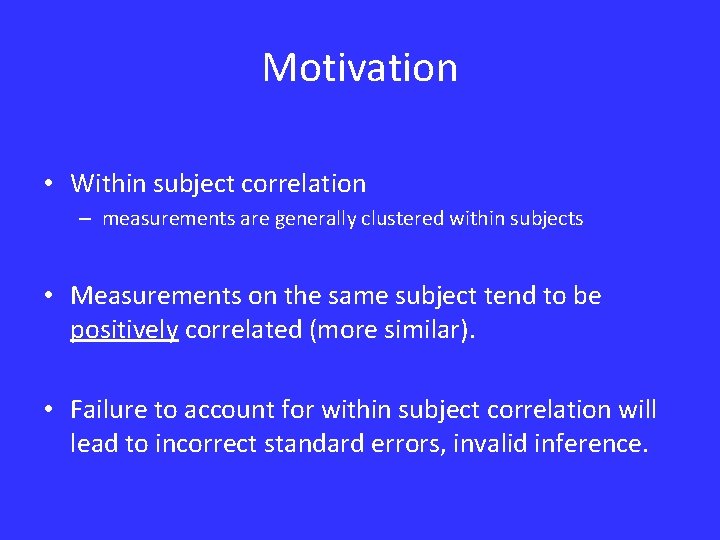
Motivation • Within subject correlation – measurements are generally clustered within subjects • Measurements on the same subject tend to be positively correlated (more similar). • Failure to account for within subject correlation will lead to incorrect standard errors, invalid inference.

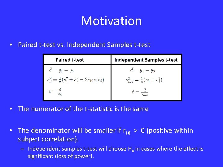
Motivation • Paired t-test vs. Independent Samples t-test • The numerator of the t-statistic is the same • The denominator will be smaller if r 10 > 0 (positive within subject correlation). – Independent samples t-test will choose H 0 in cases where the effect is significant (loss of power).

Population Average (PA) Model • Focus is on comparing the average trend over time between subpopulations. – Comparing exposure groups, treatment groups, etc… • Interpretation follows the same conventions we have developed for cross-sectional data. • Example: Is the pattern of change in an outcome the same for treatment groups?

Population Average (PA) Model • Within subject correlation is viewed as a nuisance parameter – necessary for proper inference but not typically of primary scientific interest • Primary interest usually involves between subject covariates – Covariates whose values vary across individuals in a study as opposed to within individuals.

Random Effects Model • Unobservable features of each subject’s profile represented through random effects. • All observations on a given subject share the same random effect, inducing within subject correlation. • Example: – Random Intercepts and Random slopes

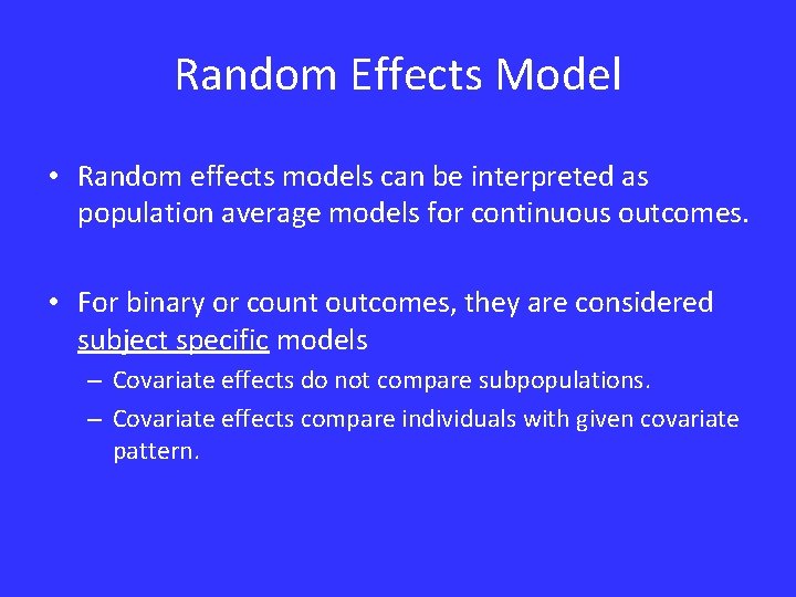
Random Effects Model • Random effects models can be interpreted as population average models for continuous outcomes. • For binary or count outcomes, they are considered subject specific models – Covariate effects do not compare subpopulations. – Covariate effects compare individuals with given covariate pattern.

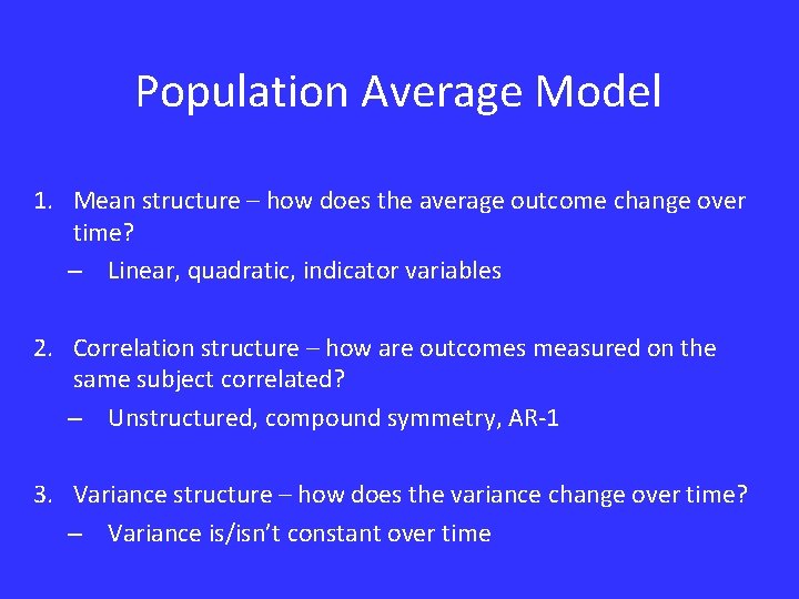
Population Average Model 1. Mean structure – how does the average outcome change over time? – Linear, quadratic, indicator variables 2. Correlation structure – how are outcomes measured on the same subject correlated? – Unstructured, compound symmetry, AR-1 3. Variance structure – how does the variance change over time? – Variance is/isn’t constant over time

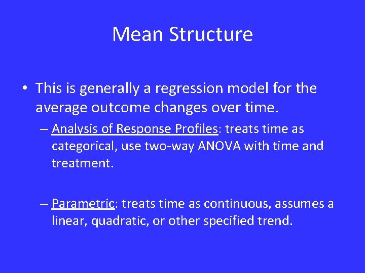
Mean Structure • This is generally a regression model for the average outcome changes over time. – Analysis of Response Profiles: treats time as categorical, use two-way ANOVA with time and treatment. – Parametric: treats time as continuous, assumes a linear, quadratic, or other specified trend.

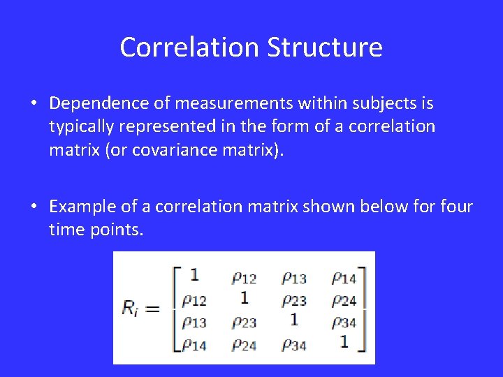
Correlation Structure • Dependence of measurements within subjects is typically represented in the form of a correlation matrix (or covariance matrix). • Example of a correlation matrix shown below for four time points.

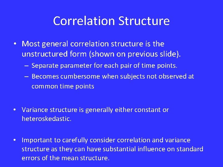
Correlation Structure • Most general correlation structure is the unstructured form (shown on previous slide). – Separate parameter for each pair of time points. – Becomes cumbersome when subjects not observed at common time points • Variance structure is generally either constant or heteroskedastic. • Important to carefully consider correlation and variance structure as they can have substantial influence on standard errors of the mean structure.

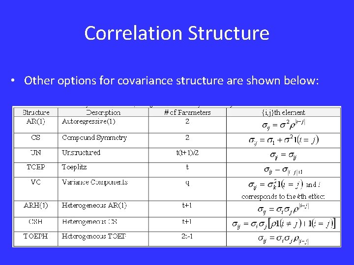
Correlation Structure • Other options for covariance structure are shown below:

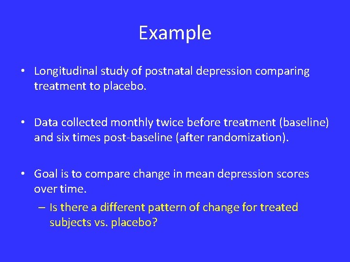
Example • Longitudinal study of postnatal depression comparing treatment to placebo. • Data collected monthly twice before treatment (baseline) and six times post-baseline (after randomization). • Goal is to compare change in mean depression scores over time. – Is there a different pattern of change for treated subjects vs. placebo?

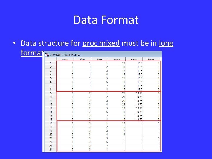
Data Format • Data structure for proc mixed must be in long format.

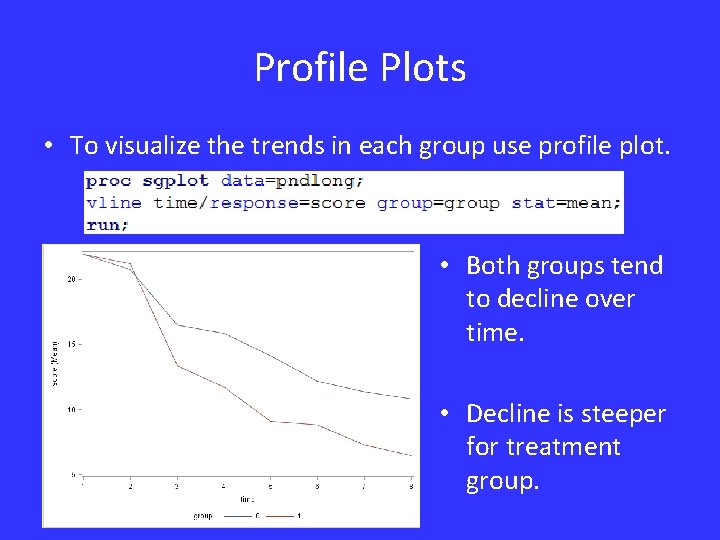
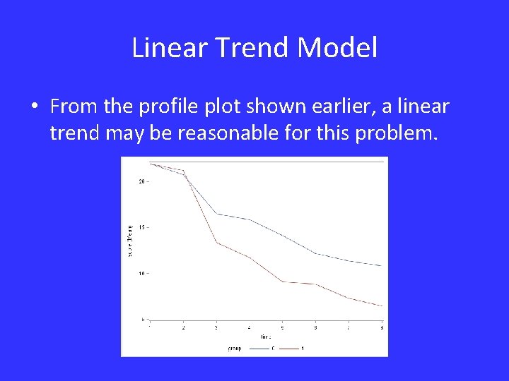
Profile Plots • To visualize the trends in each group use profile plot. • Both groups tend to decline over time. • Decline is steeper for treatment group.

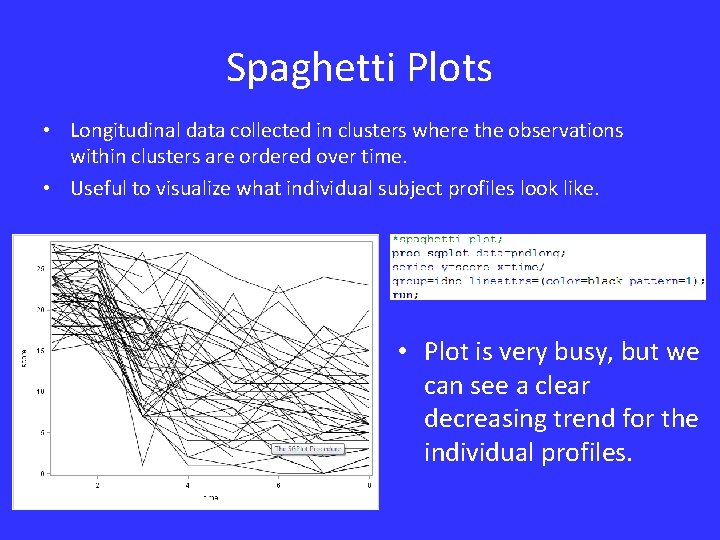
Spaghetti Plots • Longitudinal data collected in clusters where the observations within clusters are ordered over time. • Useful to visualize what individual subject profiles look like. • Plot is very busy, but we can see a clear decreasing trend for the individual profiles.

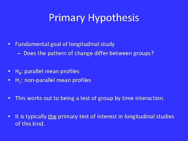
Primary Hypothesis • Fundamental goal of longitudinal study – Does the pattern of change differ between groups? • H 0: parallel mean profiles • H 1: non-parallel mean profiles • This works out to being a test of group by time interaction. • It is typically the primary test of interest in longitudinal studies of this kind.

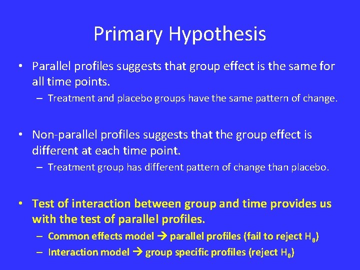
Primary Hypothesis • Parallel profiles suggests that group effect is the same for all time points. – Treatment and placebo groups have the same pattern of change. • Non-parallel profiles suggests that the group effect is different at each time point. – Treatment group has different pattern of change than placebo. • Test of interaction between group and time provides us with the test of parallel profiles. – Common effects model parallel profiles (fail to reject H 0) – Interaction model group specific profiles (reject H 0)

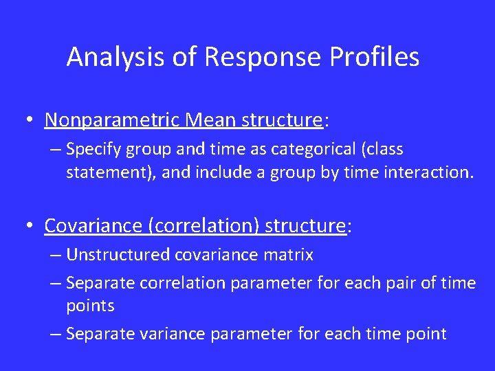
Analysis of Response Profiles • Nonparametric Mean structure: – Specify group and time as categorical (class statement), and include a group by time interaction. • Covariance (correlation) structure: – Unstructured covariance matrix – Separate correlation parameter for each pair of time points – Separate variance parameter for each time point

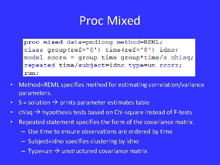
Proc Mixed • Method=REML specifies method for estimating correlation/variance parameters. • S = solution prints parameter estimates table • chisq hypothesis tests based on Chi-square instead of F-tests • Repeated statement specifies the form of the covariance matrix. – Use time to ensure observations are ordered by time – Subject=idno specifies clustering by idno – Type=un unstructured covariance matrix

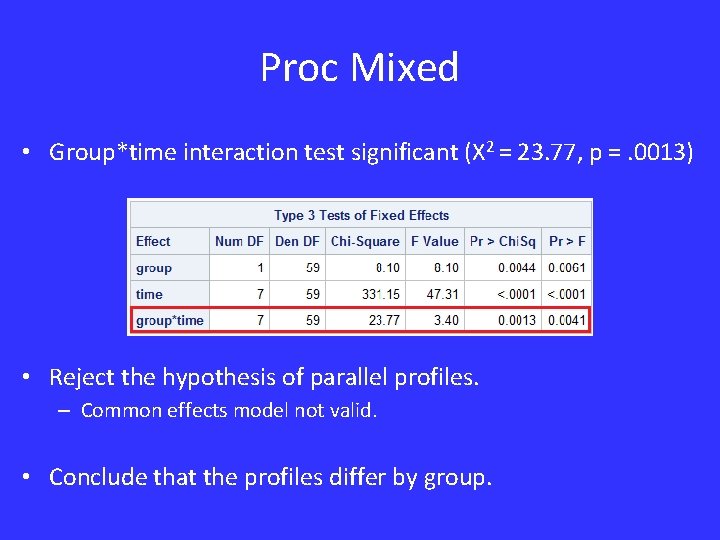
Proc Mixed • Group*time interaction test significant (X 2 = 23. 77, p =. 0013) • Reject the hypothesis of parallel profiles. – Common effects model not valid. • Conclude that the profiles differ by group.

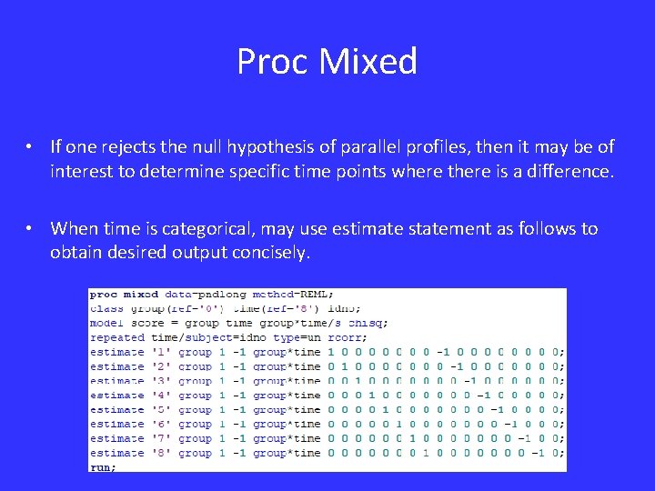
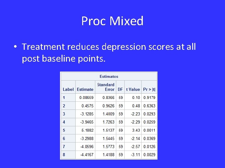
Proc Mixed • If one rejects the null hypothesis of parallel profiles, then it may be of interest to determine specific time points where there is a difference. • When time is categorical, may use estimate statement as follows to obtain desired output concisely.

Proc Mixed • Treatment reduces depression scores at all post baseline points.

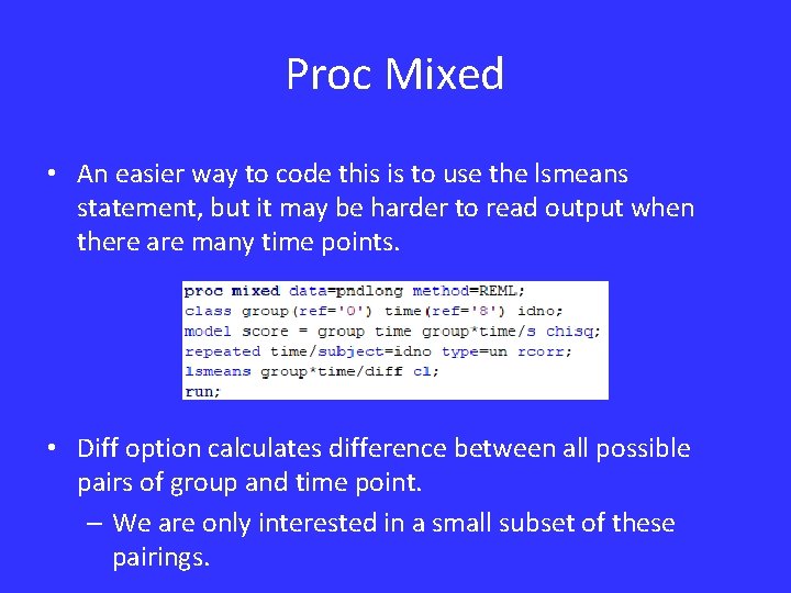
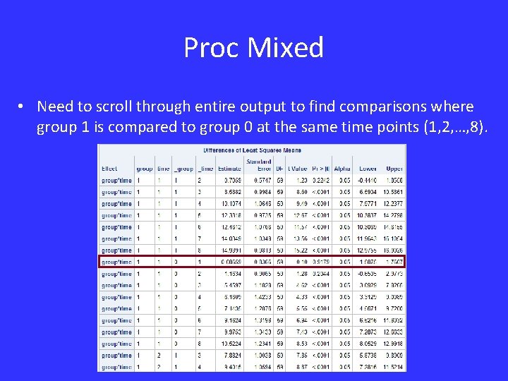
Proc Mixed • An easier way to code this is to use the lsmeans statement, but it may be harder to read output when there are many time points. • Diff option calculates difference between all possible pairs of group and time point. – We are only interested in a small subset of these pairings.

Proc Mixed • Need to scroll through entire output to find comparisons where group 1 is compared to group 0 at the same time points (1, 2, …, 8).

Linear Trend Model • The nonparametric mean structure is very flexible, captures many forms well. • Less powerful when the trend is well approximated by parametric form such as linear. • A linear trend captures the group*time interaction with one parameter, whereas the nonparametric approach requires (G-1)*(T-1).

Linear Trend Model • From the profile plot shown earlier, a linear trend may be reasonable for this problem.

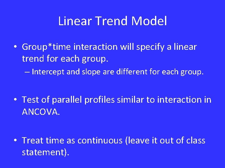
Linear Trend Model • Group*time interaction will specify a linear trend for each group. – Intercept and slope are different for each group. • Test of parallel profiles similar to interaction in ANCOVA. • Treat time as continuous (leave it out of class statement).

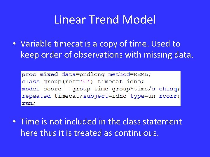
Linear Trend Model • Variable timecat is a copy of time. Used to keep order of observations with missing data. • Time is not included in the class statement here thus it is treated as continuous.

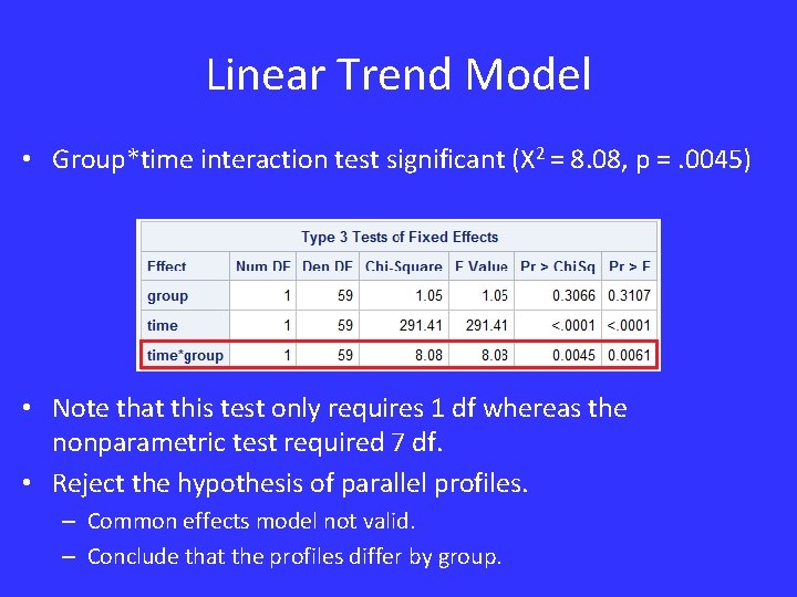
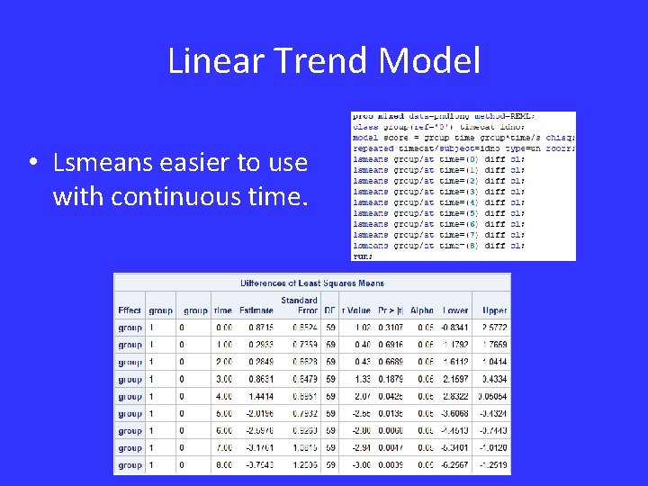
Linear Trend Model • Group*time interaction test significant (X 2 = 8. 08, p =. 0045) • Note that this test only requires 1 df whereas the nonparametric test required 7 df. • Reject the hypothesis of parallel profiles. – Common effects model not valid. – Conclude that the profiles differ by group.

Linear Trend Model • Lsmeans easier to use with continuous time.

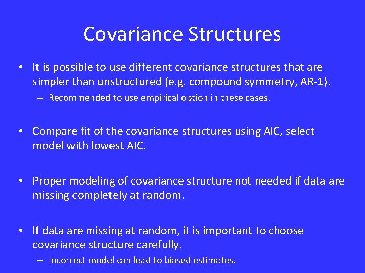
Covariance Structures • It is possible to use different covariance structures that are simpler than unstructured (e. g. compound symmetry, AR-1). – Recommended to use empirical option in these cases. • Compare fit of the covariance structures using AIC, select model with lowest AIC. • Proper modeling of covariance structure not needed if data are missing completely at random. • If data are missing at random, it is important to choose covariance structure carefully. – Incorrect model can lead to biased estimates.

Impact of Within Subject Correlation • What do we gain from modeling within subject correlation? • Showed earlier that the standard errors are reduced in the case of paired data. • Comparison to two-way ANOVA assuming independence.

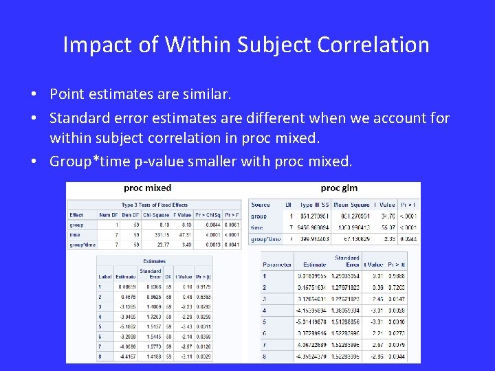
Impact of Within Subject Correlation • Point estimates are similar. • Standard error estimates are different when we account for within subject correlation in proc mixed. • Group*time p-value smaller with proc mixed.

Analysis of Response Profiles • Advantages: – Treating time as a categorical factor allows for flexible accommodation of many different trajectory shapes. – Allows a variety of within subject covariance patterns. – Can handle unbalanced data when observations are missing completely at random.

Repeated Measures Data • Disadvantages: – Cannot handle misaligned time points. – Modeling becomes cumbersome for designs with many time points (too many parameters). – If data are not missing completely at random, results may be biased. • As we’ll see next week, random effects models alleviate many of these disadvantages.