Lecture 08 Theory of Demand conclusion Lecturer Martin

Lecture # 08 Theory of Demand (conclusion) Lecturer: Martin Paredes

1. 2. 3. 4. 5. Individual Demand Curves Income and Substitution Effects and the Slope of Demand Applications: the Work-Leisure Trade-off Consumer Surplus Constructing Aggregate Demand 2

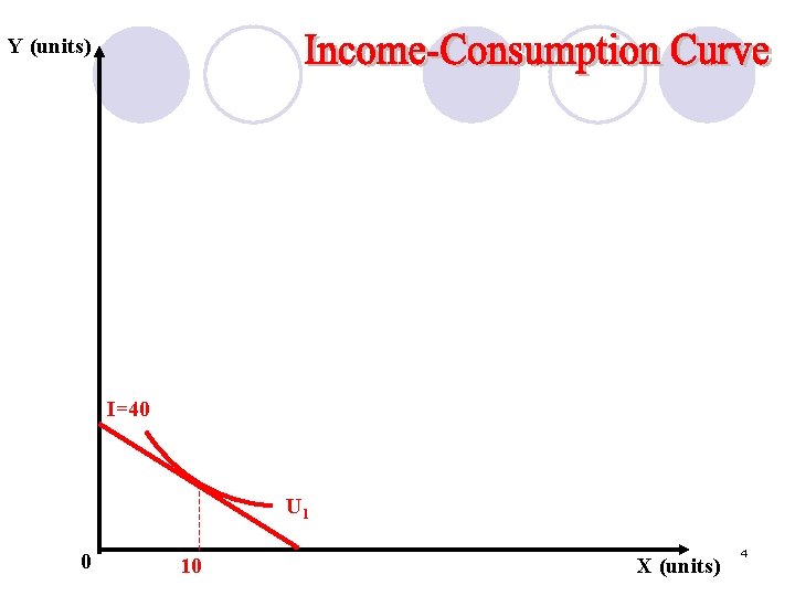
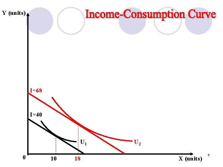
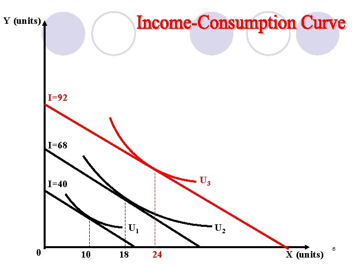
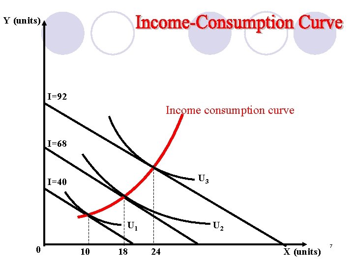
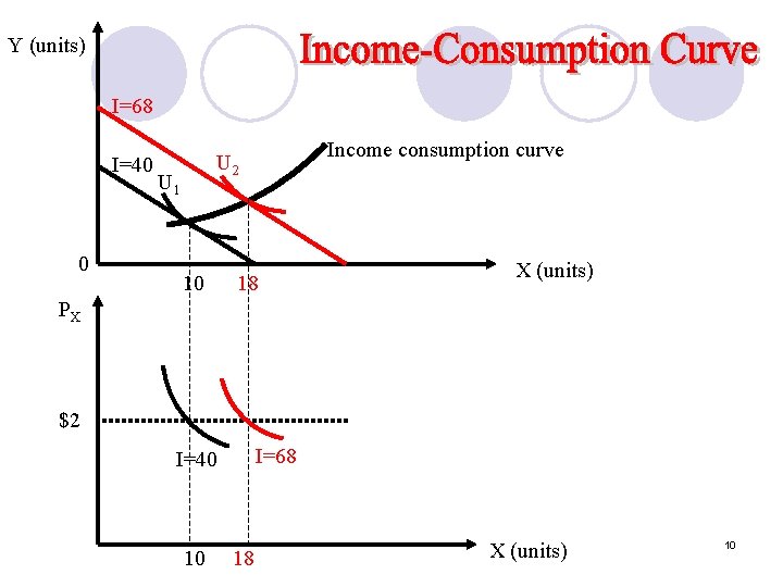
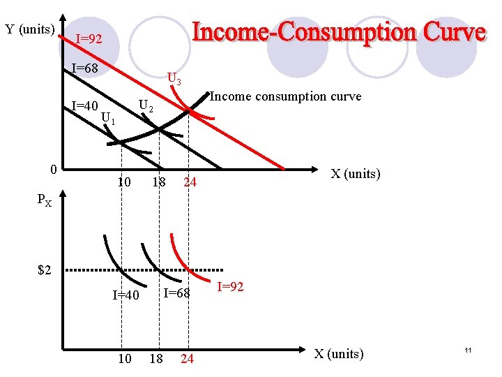
Definition: The income-consumption curve of good X is the set of optimal baskets for every possible income level. l Assumes all other variables remain constant. 3

Y (units) I=40 U 1 0 10 X (units) 4

Y (units) I=68 I=40 U 1 0 10 18 U 2 X (units) 5

Y (units) I=92 I=68 U 3 I=40 U 1 0 10 18 U 2 24 X (units) 6

Y (units) I=92 Income consumption curve I=68 U 3 I=40 U 1 0 10 18 U 2 24 X (units) 7

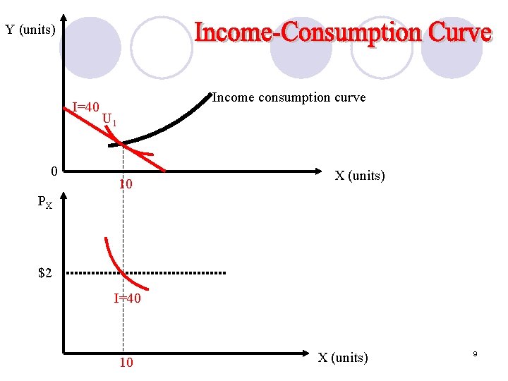
Note: l The points on the income-consumption curve can be graphed as points on a shifting demand curve. 8

Y (units) I=40 0 Income consumption curve U 1 10 X (units) PX $2 I=40 10 X (units) 9

Y (units) I=68 I=40 0 Income consumption curve U 2 U 1 10 18 X (units) PX $2 I=68 I=40 10 18 X (units) 10

Y (units) I=92 I=68 I=40 0 U 3 Income consumption curve U 2 U 1 10 18 X (units) 24 PX $2 I=68 I=40 10 18 24 I=92 X (units) 11

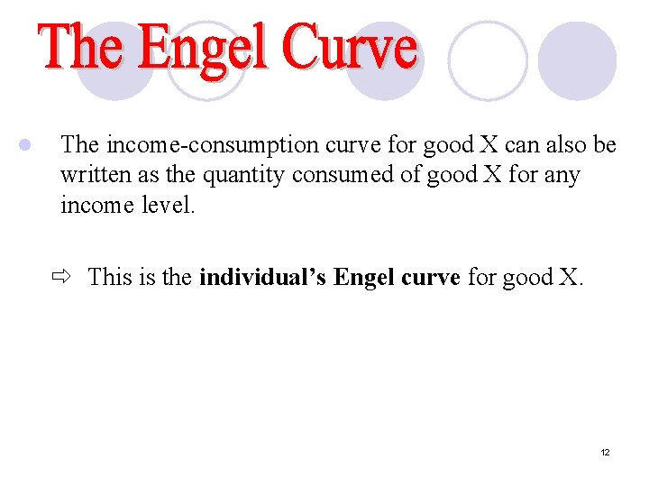
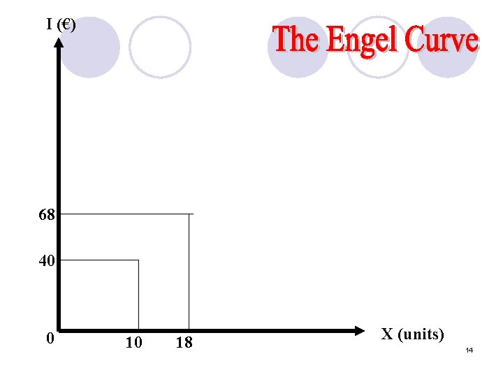
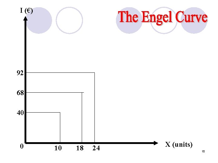
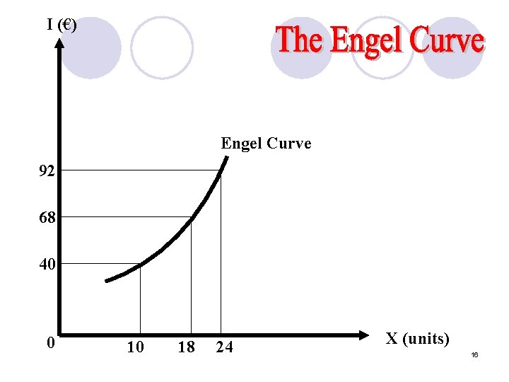
l The income-consumption curve for good X can also be written as the quantity consumed of good X for any income level. ð This is the individual’s Engel curve for good X. 12

I (€) 40 0 10 X (units) 13

I (€) 68 40 0 10 18 X (units) 14

I (€) 92 68 40 0 10 18 24 X (units) 15

I (€) Engel Curve 92 68 40 0 10 18 24 X (units) 16

Note: l When the slope of the income-consumption curve is positive, then the slope of the Engel curve is also positive. 17

Normal Good: l If the income consumption curve shows that the consumer purchases more of good X as her income rises, good X is a normal good. l Equivalently, if the slope of the Engel curve is positive, the good is a normal good. 18

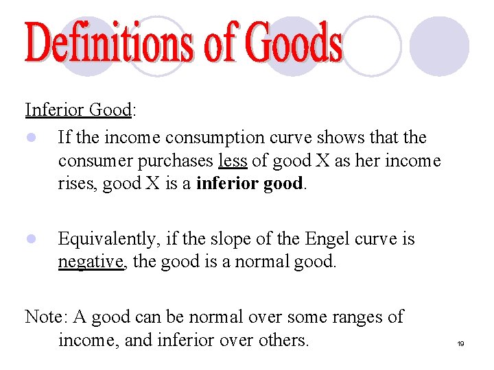
Inferior Good: l If the income consumption curve shows that the consumer purchases less of good X as her income rises, good X is a inferior good. l Equivalently, if the slope of the Engel curve is negative, the good is a normal good. Note: A good can be normal over some ranges of income, and inferior over others. 19

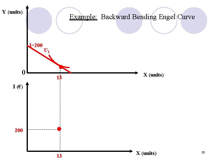
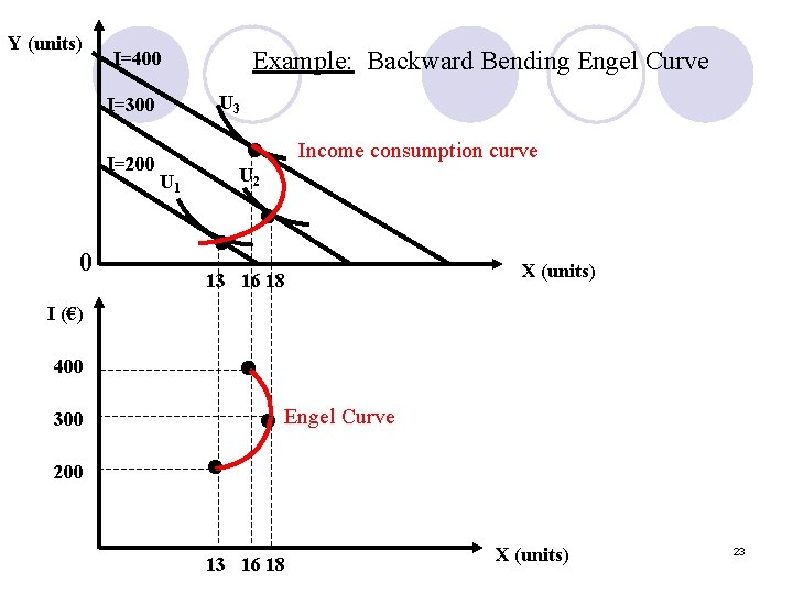
Y (units) Example: Backward Bending Engel Curve I=200 0 U 1 • 13 X (units) I (€) 200 • 13 X (units) 20

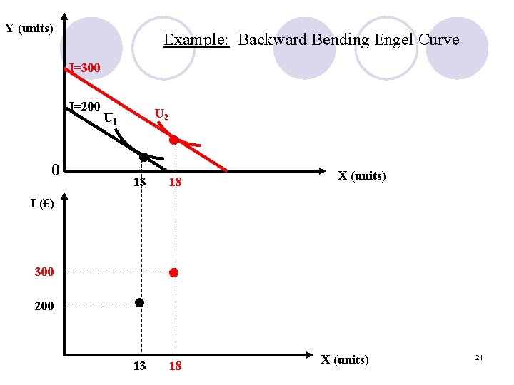
Y (units) Example: Backward Bending Engel Curve I=300 I=200 0 U 1 U 2 • • 13 18 X (units) I (€) 300 200 • 13 • 18 X (units) 21

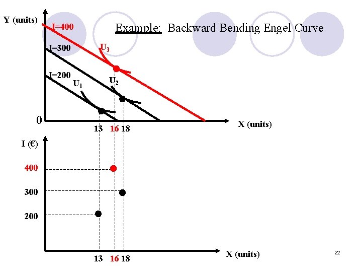
Y (units) U 3 I=300 I=200 0 Example: Backward Bending Engel Curve I=400 U 1 • • • U 2 13 16 18 X (units) I (€) • 400 300 200 • • 13 16 18 X (units) 22

Y (units) U 3 I=300 I=200 0 Example: Backward Bending Engel Curve I=400 U 1 • • • Income consumption curve U 2 13 16 18 X (units) I (€) • 400 300 200 • • Engel Curve 13 16 18 X (units) 23

l There are two effects: 1. Income Effect 2. Substitution Effect 24

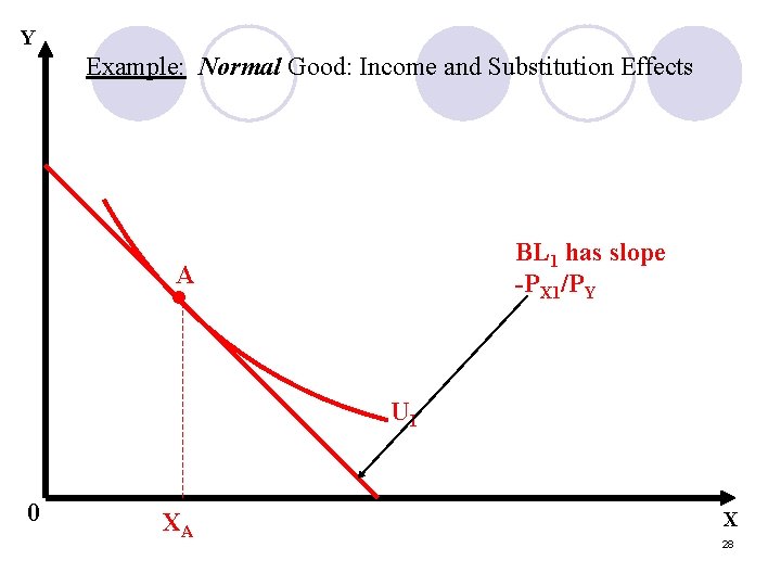
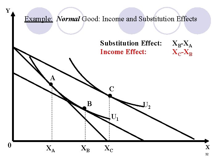
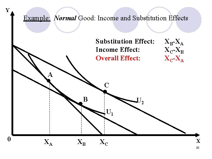
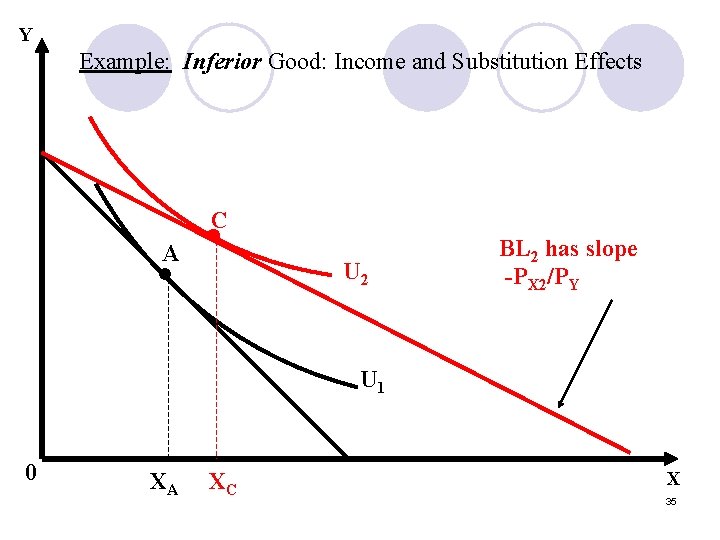
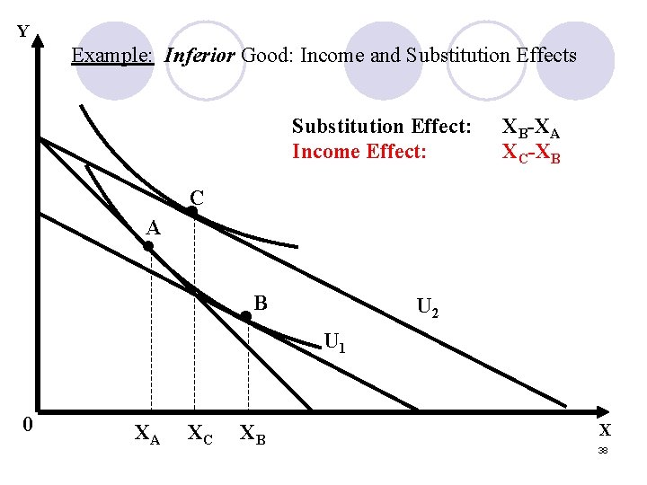
Definition: When the price of good X falls, purchasing power rises. This is called the income effect of a change in price. l l It assumes all else remain constant The income effect may be: 1. Positive (normal good) 2. Negative (inferior good). 25

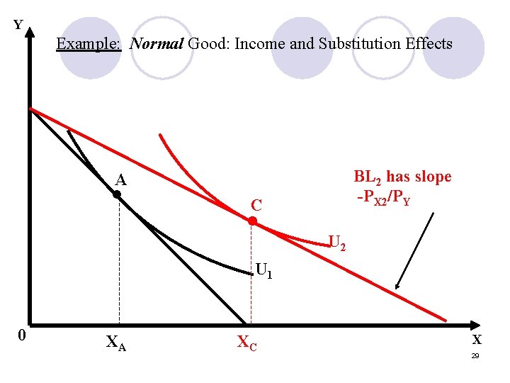
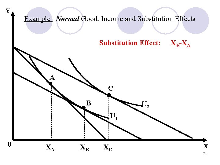
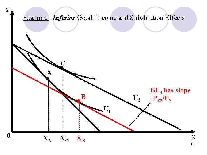
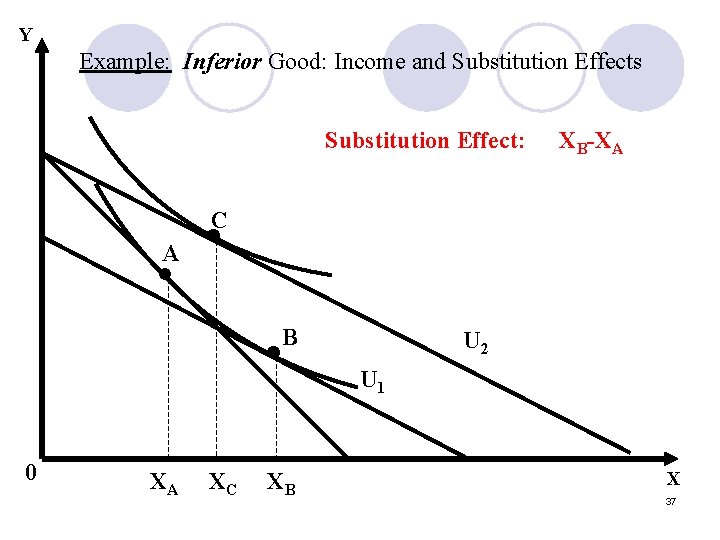
Definition: When the price of good X falls, good X becomes cheaper relative to good Y. This change in relative prices alone causes the consumer to adjust his consumption basket. This effect is called the substitution effect. l It assumes all else remain constant l The substitution effect is always negative 26

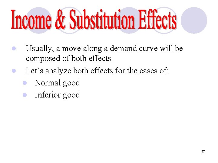
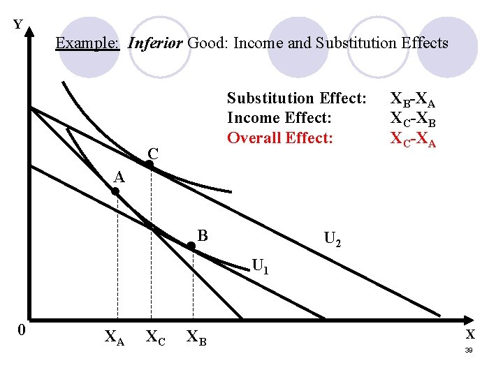
Usually, a move along a demand curve will be composed of both effects. l Let’s analyze both effects for the cases of: l Normal good l Inferior good l 27

Y Example: Normal Good: Income and Substitution Effects BL 1 has slope -PX 1/PY A • U 1 0 XA X 28

Y Example: Normal Good: Income and Substitution Effects BL 2 has slope -PX 2/PY A • C • U 2 U 1 0 XA XC X 29

Y Example: Normal Good: Income and Substitution Effects A • C B • 0 XA XB • U 2 BLd has slope -PX 2/PY U 1 XC X 30

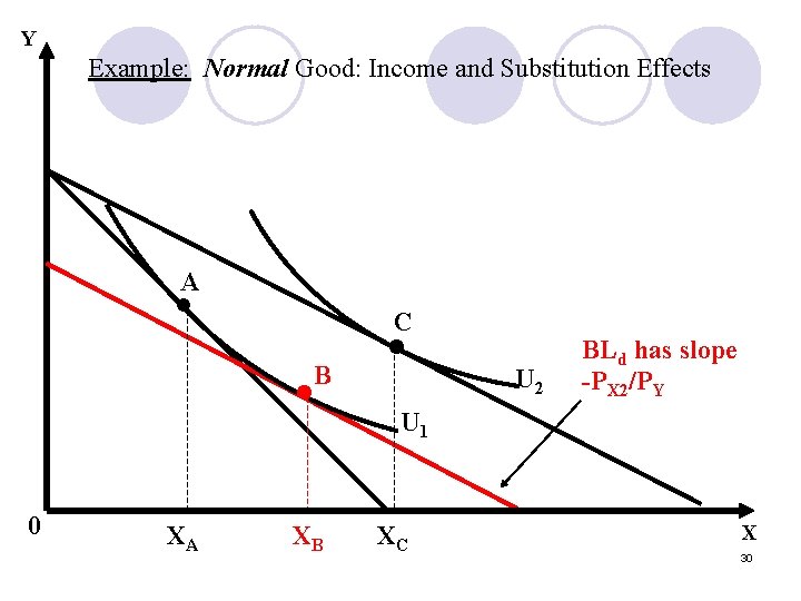
Y Example: Normal Good: Income and Substitution Effects Substitution Effect: XB-XA A • C B • 0 XA XB • U 2 U 1 XC X 31

Y Example: Normal Good: Income and Substitution Effects Substitution Effect: Income Effect: XB-XA XC-XB A • C B • 0 XA XB • U 2 U 1 XC X 32

Y Example: Normal Good: Income and Substitution Effects Substitution Effect: Income Effect: Overall Effect: XB-XA XC-XB XC-XA A • C B • 0 XA XB • U 2 U 1 XC X 33

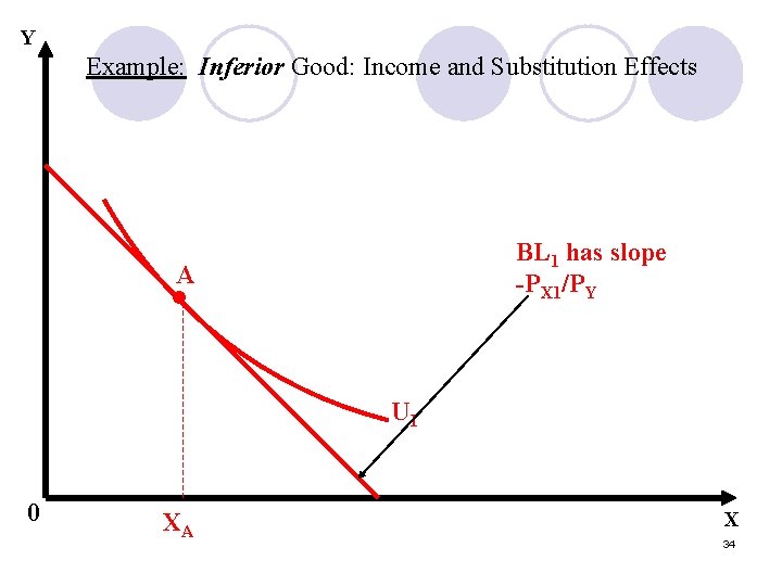
Y Example: Inferior Good: Income and Substitution Effects BL 1 has slope -PX 1/PY A • U 1 0 XA X 34

Y Example: Inferior Good: Income and Substitution Effects C A • • U 2 BL 2 has slope -PX 2/PY U 1 0 XA XC X 35

Y Example: Inferior Good: Income and Substitution Effects C A • • B • 0 XA XC XB U 2 BLd has slope -PX 2/PY U 1 X 36

Y Example: Inferior Good: Income and Substitution Effects Substitution Effect: XB-XA C A • • B • 0 XA XC XB U 2 U 1 X 37

Y Example: Inferior Good: Income and Substitution Effects Substitution Effect: Income Effect: XB-XA XC-XB C A • • B • 0 XA XC XB U 2 U 1 X 38

Y Example: Inferior Good: Income and Substitution Effects Substitution Effect: Income Effect: Overall Effect: C A • • B • 0 XA XC XB XB-XA XC-XB XC-XA U 2 U 1 X 39

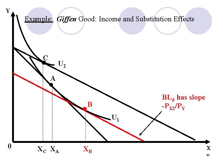
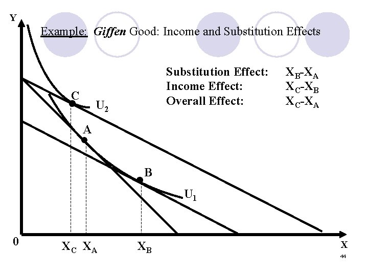
l l Theoretically, it is possible that, for an inferior good, the income effect dominates the substitution effect A Giffen good is a good that is so inferior, that the net effect of a decrease in the price of that good, all else constant, is a decrease in consumption of that good. 40

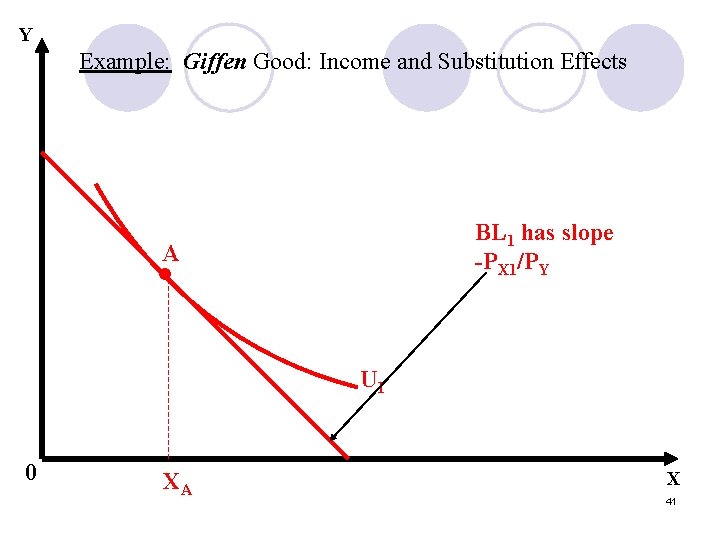
Y Example: Giffen Good: Income and Substitution Effects BL 1 has slope -PX 1/PY A • U 1 0 XA X 41

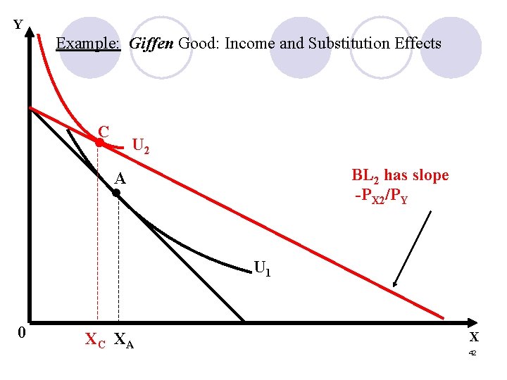
Y Example: Giffen Good: Income and Substitution Effects C • U 2 BL 2 has slope -PX 2/PY A • U 1 0 XC XA X 42

Y Example: Giffen Good: Income and Substitution Effects C • U 2 A • BLd has slope -PX 2/PY B • 0 XC XA XB U 1 X 43

Y Example: Giffen Good: Income and Substitution Effects C • Substitution Effect: Income Effect: Overall Effect: U 2 XB-XA XC-XB XC-XA A • B • 0 XC XA XB U 1 X 44

Notes: l For Giffen goods, demand does not slope down. l For the income effect to be large enough to offset the substitution effect, the good would have to represent a very large proportion of the budget. 45

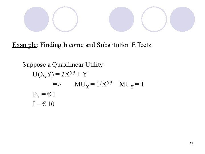
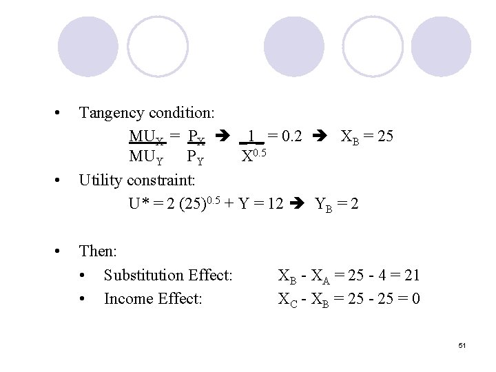
Example: Finding Income and Substitution Effects Suppose a Quasilinear Utility: U(X, Y) = 2 X 0. 5 + Y => MUX = 1/X 0. 5 PY = € 1 I = € 10 MUY = 1 46

1. Suppose PX = € 0. 50 • Tangency condition: MUX = PX _1_ = 0. 5 XA = 4 MUY PY X 0. 5 • Budget constraint: PX. X + P Y. Y = I YA = 8 • Utility level: U* = 2 (4)0. 5 + 8 = 12 47

2. Suppose PX = € 0. 20 • Tangency condition: MUX = PX _1_ = 0. 2 XC = 25 MUY PY X 0. 5 • Budget constraint: PX. X + P Y. Y = I YC = 5 • Utility level: U* = 2 (25)0. 5 + 5 = 15 48

3. What are the substitution and income effects that result from the decline in PX? • Find the basket B that gives a utility level of U = 12 at prices PX = € 0. 20 and PY = € 1 49

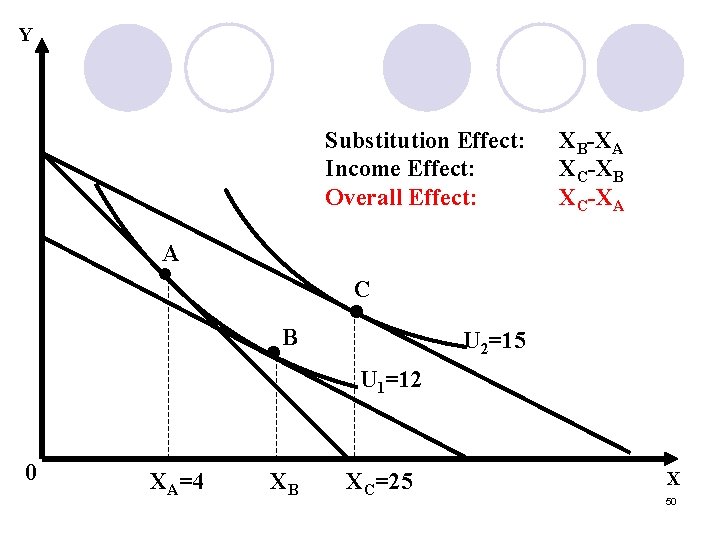
Y Substitution Effect: Income Effect: Overall Effect: XB-XA XC-XB XC-XA A • C B • 0 XA=4 XB • U 2=15 U 1=12 XC=25 X 50

• • • Tangency condition: MUX = PX _1_ = 0. 2 XB = 25 MUY PY X 0. 5 Utility constraint: U* = 2 (25)0. 5 + Y = 12 YB = 2 Then: • Substitution Effect: • Income Effect: XB - XA = 25 - 4 = 21 XC - XB = 25 - 25 = 0 51

l l The individual’s demand curve can be interpreted as the maximum amount such individual is willing to pay for a good In turn, the market price determines the amount the individual actually pays for all the units consumed. 52

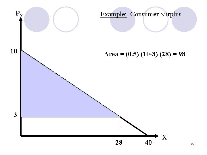
Definition: l The consumer surplus is the net economic benefit to the consumer due to a purchase of a good l It is measured by the difference between the maximum amount the consumer is willing to pay and the actual amount he pays for it. l The area under the ordinary demand curve and above the market price provides a measure of consumer surplus. 53

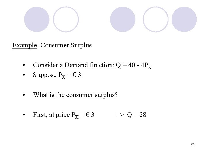
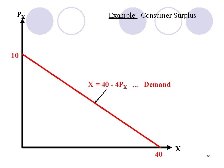
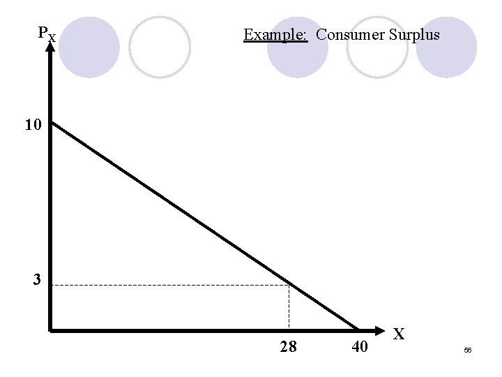
Example: Consumer Surplus • • Consider a Demand function: Q = 40 - 4 PX Suppose PX = € 3 • What is the consumer surplus? • First, at price PX = € 3 => Q = 28 54

PX Example: Consumer Surplus 10 X = 40 - 4 PX. . . Demand 40 X 55

PX Example: Consumer Surplus 10 3 28 40 X 56

PX Example: Consumer Surplus 10 Area = (0. 5) (10 -3) (28) = 98 G 3 28 40 X 57

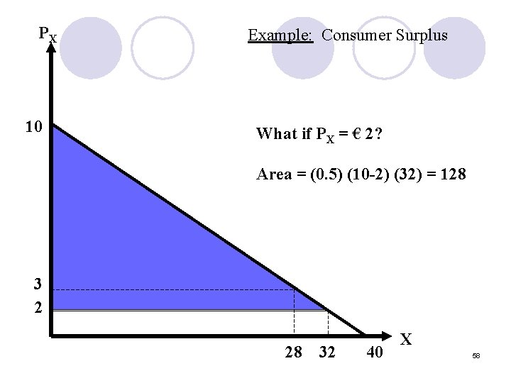
PX 10 Example: Consumer Surplus What if PX = € 2? Area = (0. 5) (10 -2) (32) = 128 3 2 28 32 40 X 58

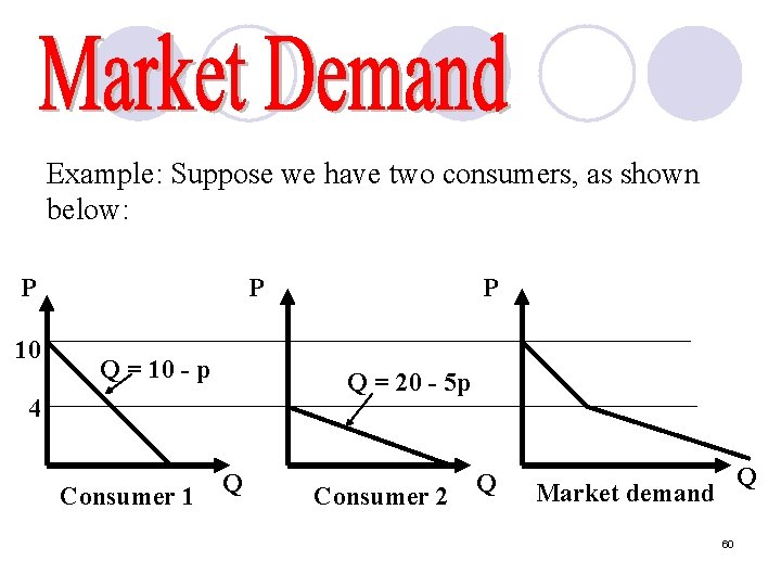
Definition: The market demand function is the horizontal sum of the demands of the individual consumers. l In other words, the market demand is obtained by adding the quantities demanded by the individuals at each price and plotting this total quantity for all possible prices. 59

Example: Suppose we have two consumers, as shown below: P 10 P Q = 10 - p Q = 20 - 5 p 4 Consumer 1 P Q Consumer 2 Q Q Market demand 60

1. Individual ordinary (uncompensated) demands are derived from the utility maximization problem of the consumer. 2. The optimal consumption basket for a utility maximizing consumer changes as prices change due to both income and substitution effects. 61

3. If income effects are strong enough, a price rise may result in increased consumption for an optimizing consumer. 4. Consumer surplus measures the net economic benefit of a purchase. 5. Market demand is the horizontal sum of the individual consumer demands for a particular good. 62