Introduction to Computational Natural Language Learning Linguistics 79400

Introduction to Computational Natural Language Learning Linguistics 79400 (Under: Topics in Natural Language Processing) Computer Science 83000 (Under: Topics in Artificial Intelligence) The Graduate School of the City University of New York Fall 2001 William Gregory Sakas Hunter College, Department of Computer Science Graduate Center, Ph. D Programs in Computer Science and Linguistics The City University of New York 1

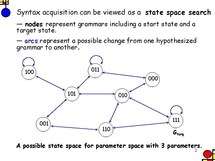
Syntax acquisition can be viewed as a state space search — nodes represent grammars including a start state and a target state. — arcs represent a possible change from one hypothesized grammar to another. 011 100 000 101 010 111 110 Gtarg A possible state space for parameter space with 3 parameters. 2

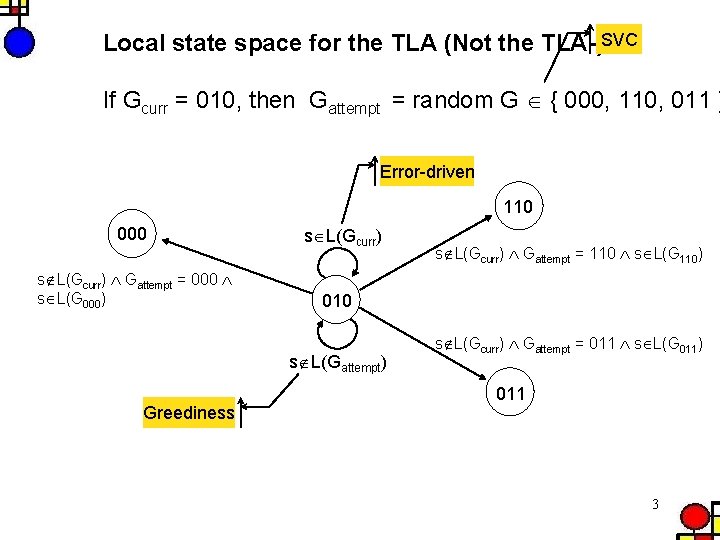
Local state space for the TLA (Not the TLA-)SVC If Gcurr = 010, then Gattempt = random G { 000, 110, 011 } Error-driven 110 000 s L(Gcurr) Gattempt = 000 s L(G 000) s L(Gcurr) 010 s L(Gattempt) Greediness s L(Gcurr) Gattempt = 110 s L(G 110) s L(Gcurr) Gattempt = 011 s L(G 011) 011 3

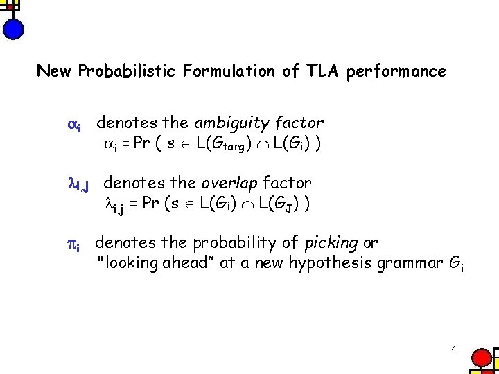
New Probabilistic Formulation of TLA performance i denotes the ambiguity factor i = Pr ( s L(Gtarg) L(Gi) ) i, j denotes the overlap factor i, j = Pr (s L(Gi) L(GJ) ) i denotes the probability of picking or "looking ahead” at a new hypothesis grammar G i 4

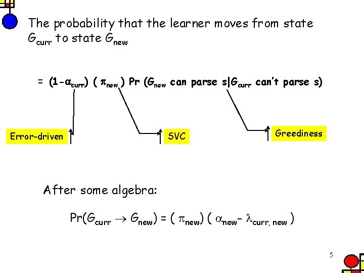
The probability that the learner moves from state Gcurr to state Gnew = (1 - curr) ( new ) Pr (Gnew can parse s|Gcurr can’t parse s) Error-driven SVC Greediness After some algebra: Pr(Gcurr Gnew) = ( new) ( new- curr, new ) 5

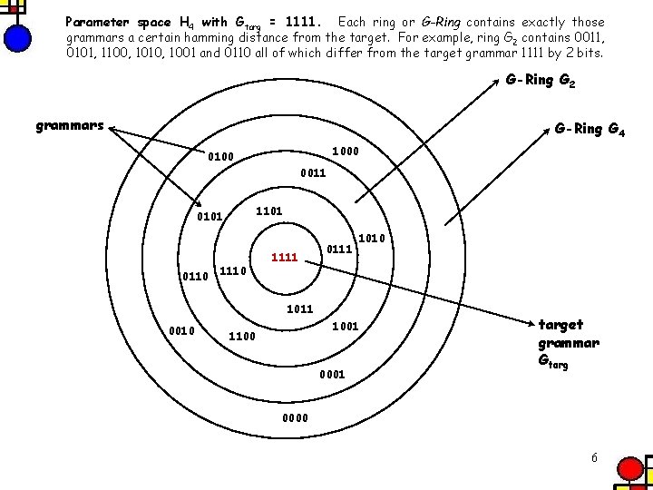
Parameter space H 4 with Gtarg = 1111. Each ring or G-Ring contains exactly those grammars a certain hamming distance from the target. For example, ring G 2 contains 0011, 0101, 1100, 1010, 1001 and 0110 all of which differ from the target grammar 1111 by 2 bits. G-Ring G 2 grammars G-Ring G 4 1000 0100 0011 1101 0110 1111 0111 1010 1011 0010 1001 1100 0001 target grammar Gtarg 0000 6

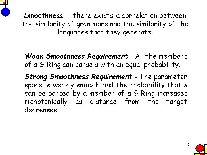
Smoothness - there exists a correlation between the similarity of grammars and the similarity of the languages that they generate. Weak Smoothness Requirement - All the members of a G-Ring can parse s with an equal probability. Strong Smoothness Requirement - The parameter space is weakly smooth and the probability that s can be parsed by a member of a G-Ring increases monotonically as distance from the target decreases. 7

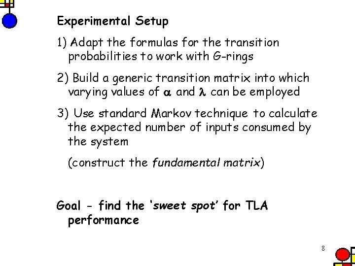
Experimental Setup 1) Adapt the formulas for the transition probabilities to work with G-rings 2) Build a generic transition matrix into which varying values of and can be employed 3) Use standard Markov technique to calculate the expected number of inputs consumed by the system (construct the fundamental matrix) Goal - find the ‘sweet spot’ for TLA performance 8

Three experiments 1) G-Rings equally likely to parse an input sentence (uniform domain) 2) G-Rings are strongly smooth (smooth domain) 3) Anything goes domain Problem: How to find combinations of and that are optimal? Solution: Use an an optimization algorithm: GRG 2 (Lasdon and Waren, 1978). 9

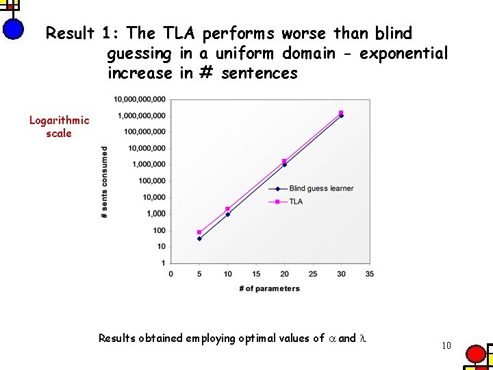
Result 1: The TLA performs worse than blind guessing in a uniform domain - exponential increase in # sentences Logarithmic scale Results obtained employing optimal values of and 10

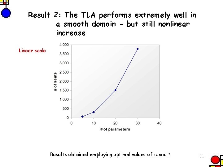
Result 2: The TLA performs extremely well in a smooth domain - but still nonlinear increase Linear scale Results obtained employing optimal values of and 11

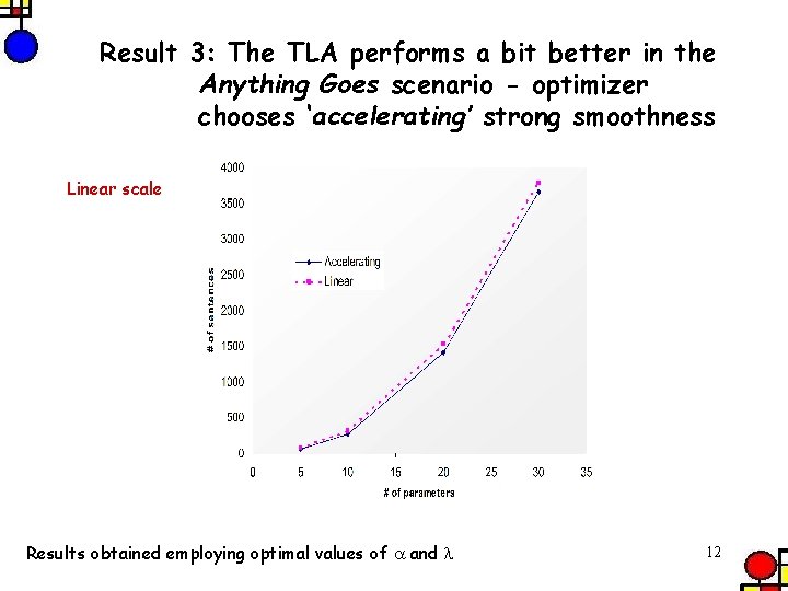
Result 3: The TLA performs a bit better in the Anything Goes scenario - optimizer chooses ‘accelerating’ strong smoothness Linear scale Results obtained employing optimal values of and 12

In summary TLA is an infeasible learner: With cross-language ambiguity uniformly distributed across the domain of languages, the number of sentences required by the number of sentences consumed by the TLA is exponential in the number of parameters. TLA is a feasible learner: In strongly smooth domains, the number of sentences increases at a rate much closer to linear as the number of parameters increases (i. e. the number of grammars increases exponentially). 13

A second case study: The Structural Triggers Learner (Fodor 1998) 14

The Parametric Principle - (Fodor 1995, 1998; Sakas and Fodor, 2001) Set individual parameters. Do not evaluate whole grammars. Halves the size of the grammar pool with each successful learning event. e. g. When 5 of 30 parameters are set 3% of grammar pool remains 15

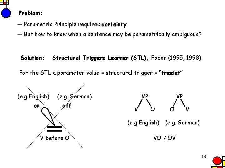
Problem: — Parametric Principle requires certainty — But how to know when a sentence may be parametrically ambiguous? Solution: Structural Triggers Learner (STL), Fodor (1995, 1998) For the STL a parameter value = structural trigger = “treelet” (e. g English) on (e. g. German) off VP V VP O (e. g English) V before O O V (e. g. German) VO / OV 16

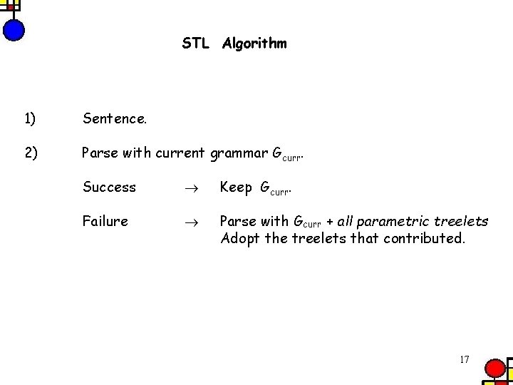
STL Algorithm 1) Sentence. 2) Parse with current grammar Gcurr. Success Keep Gcurr. Failure Parse with Gcurr + all parametric treelets Adopt the treelets that contributed. 17

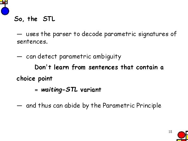
So, the STL — uses the parser to decode parametric signatures of sentences. — can detect parametric ambiguity Don't learn from sentences that contain a choice point = waiting-STL variant — and thus can abide by the Parametric Principle 18

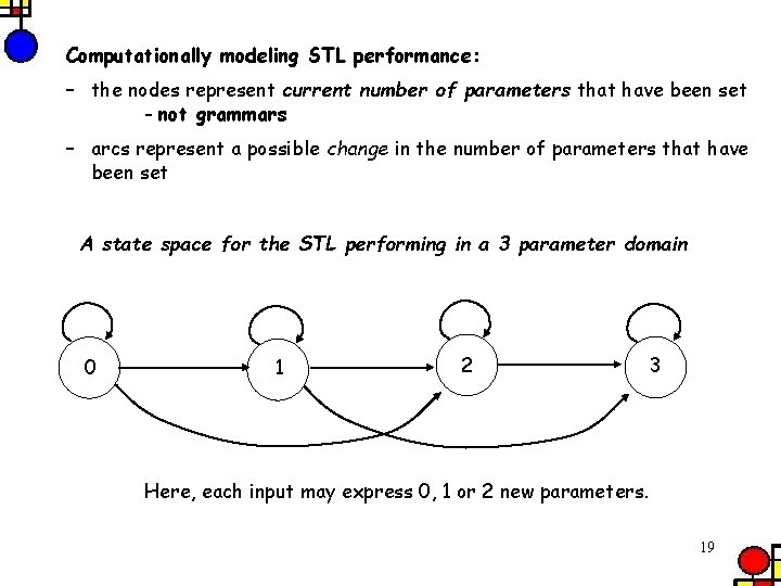
Computationally modeling STL performance: – the nodes represent current number of parameters that have been set - not grammars – arcs represent a possible change in the number of parameters that have been set A state space for the STL performing in a 3 parameter domain 0 1 2 3 Here, each input may express 0, 1 or 2 new parameters. 19

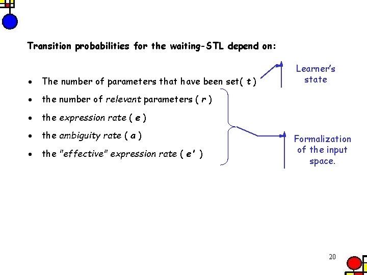
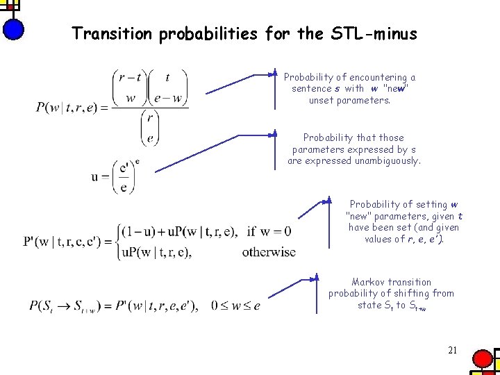
Transition probabilities for the waiting-STL depend on: · The number of parameters that have been set( t ) Learner’s state · the number of relevant parameters ( r ) · the expression rate ( e ) · the ambiguity rate ( a ) · the "effective" expression rate ( e' ) Formalization of the input space. 20

Transition probabilities for the STL-minus Probability of encountering a sentence s with w "new" unset parameters. Probability that those parameters expressed by s are expressed unambiguously. Probability of setting w "new" parameters, given t have been set (and given values of r, e, e'). Markov transition probability of shifting from state St to St+w 21

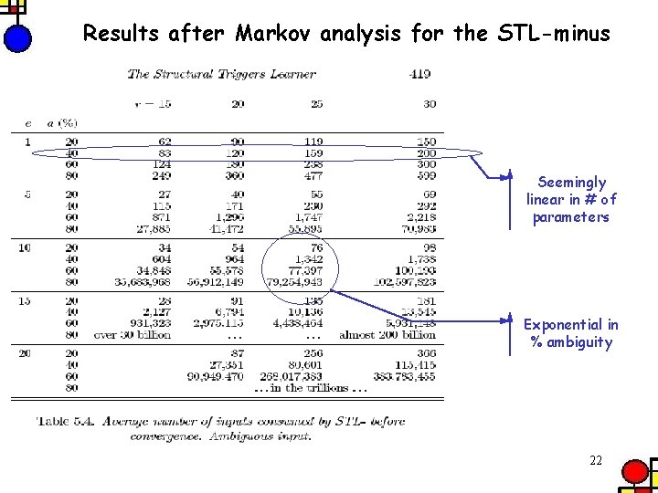
Results after Markov analysis for the STL-minus Seemingly linear in # of parameters Exponential in % ambiguity 22

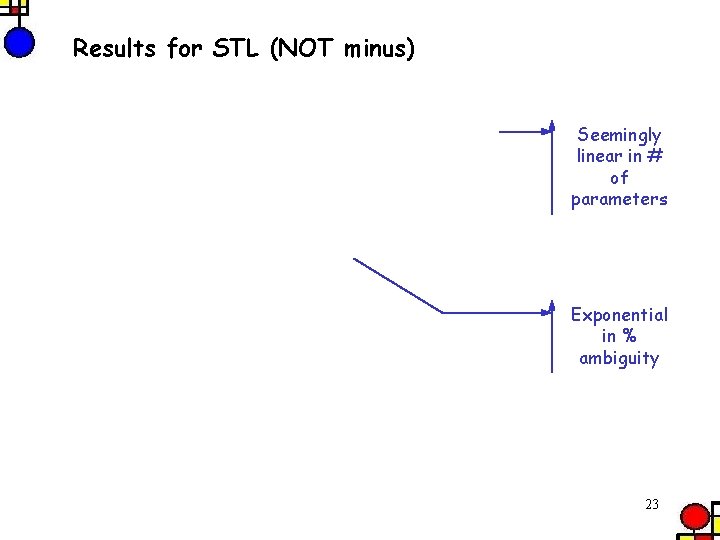
Results for STL (NOT minus) Seemingly linear in # of parameters Exponential in % ambiguity 23

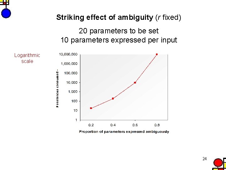
Striking effect of ambiguity (r fixed) 20 parameters to be set 10 parameters expressed per input Logarithmic scale 24

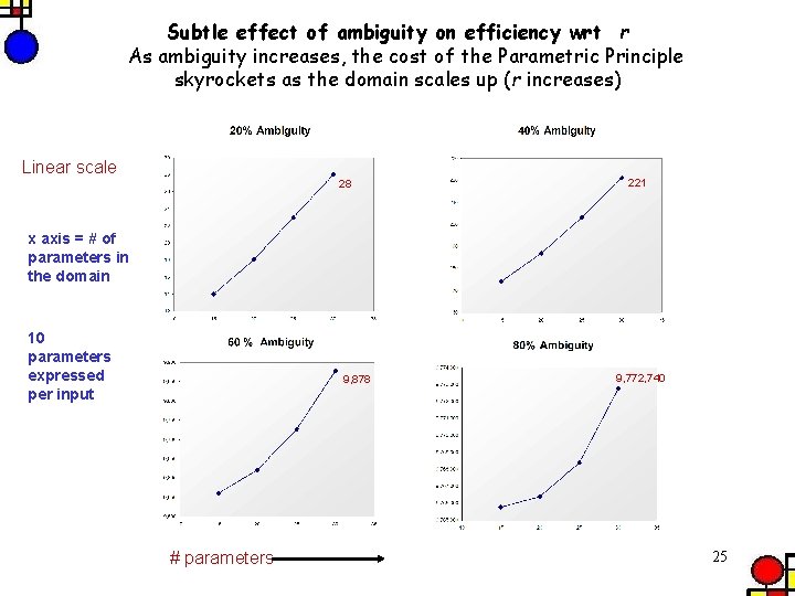
Subtle effect of ambiguity on efficiency wrt r As ambiguity increases, the cost of the Parametric Principle skyrockets as the domain scales up (r increases) Linear scale 28 221 x axis = # of parameters in the domain 10 parameters expressed per input 9, 878 # parameters 9, 772, 740 25

The effect of ambiguity (interacting with e and r) How / where is the cost incurred? By far the greatest amount of damage inflicted by ambiguity occurs at the very earliest stages of learning the wait for the first fully unambiguous trigger + a little wait for sentences that express the last few parameters unambiguously 26

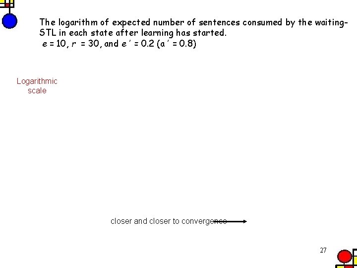
The logarithm of expected number of sentences consumed by the waiting. STL in each state after learning has started. e = 10, r = 30, and e΄ = 0. 2 (a΄ = 0. 8) Logarithmic scale closer and closer to convergence 27

STL — Bad News Ambiguity is damaging even to a parametrically-principled learner Abiding by the Parametric Principle does not, in and of itself, guarantee merely linear increase in the complexity of the learning task as the number of parameters increases. . 28

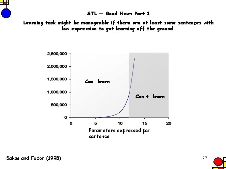
STL — Good News Part 1 Learning task might be manageable if there at least some sentences with low expression to get learning off the ground. Can learn Can't learn Parameters expressed per sentence Sakas and Fodor (1998) 29

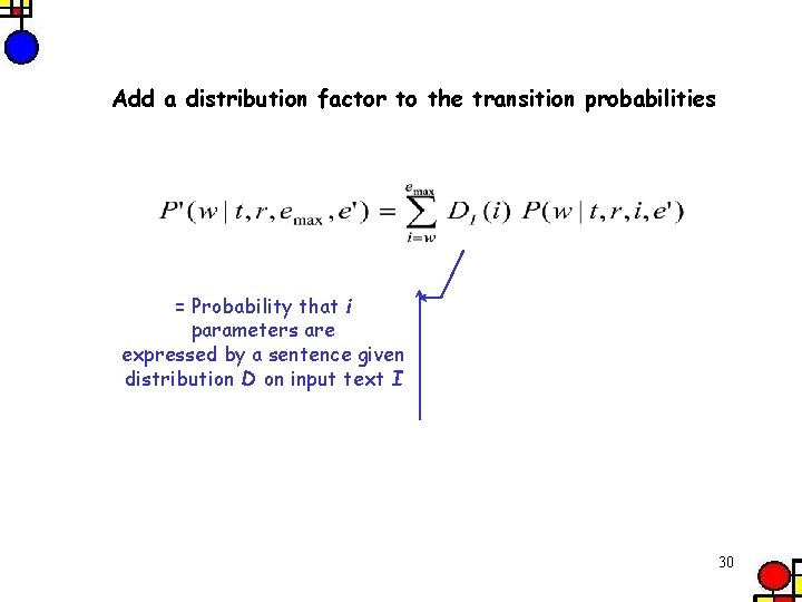
Add a distribution factor to the transition probabilities = Probability that i parameters are expressed by a sentence given distribution D on input text I 30

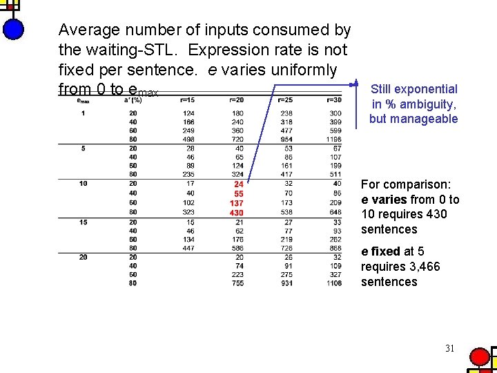
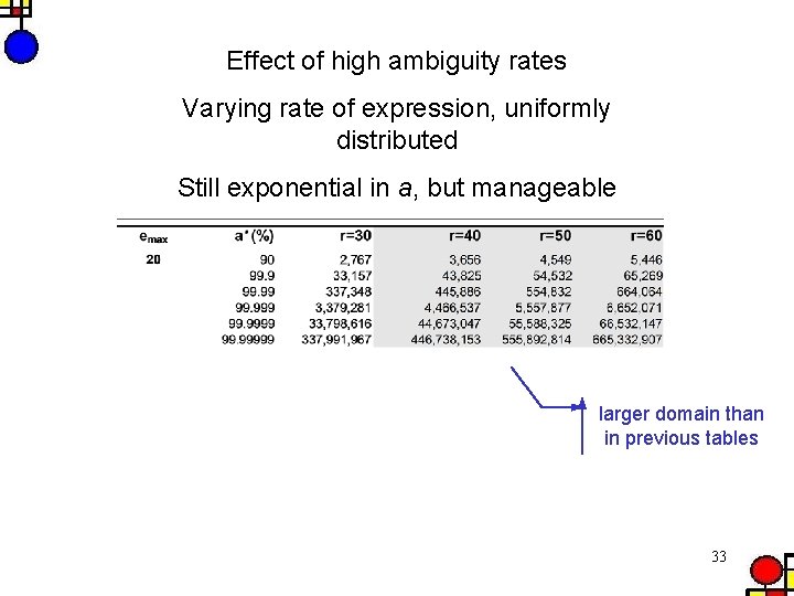
Average number of inputs consumed by the waiting-STL. Expression rate is not fixed per sentence. e varies uniformly from 0 to emax Still exponential in % ambiguity, but manageable For comparison: e varies from 0 to 10 requires 430 sentences e fixed at 5 requires 3, 466 sentences 31

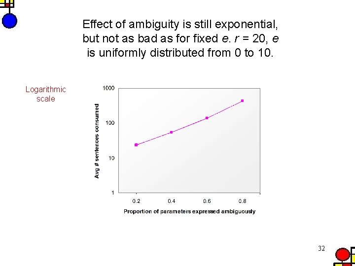
Effect of ambiguity is still exponential, but not as bad as for fixed e. r = 20, e is uniformly distributed from 0 to 10. Logarithmic scale 32

Effect of high ambiguity rates Varying rate of expression, uniformly distributed Still exponential in a, but manageable larger domain than in previous tables 33

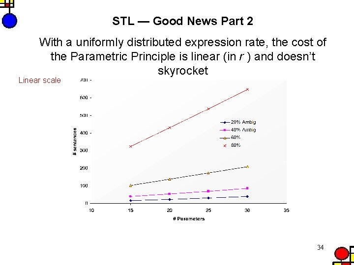
STL — Good News Part 2 With a uniformly distributed expression rate, the cost of the Parametric Principle is linear (in r ) and doesn’t skyrocket Linear scale 34

In summary: With a uniformly distributed expression rate, the number of sentences required by the STL falls in a manageable range (though still exponential in % ambiguity) The number of sentences increases only linearly as the number of parameters increases (i. e. the number of grammars increases exponentially). 35

No Best Strategy Conjecture (roughly in the spirit of Schaffer, 1994): Algorithms may be extremely efficient in specific domains, but not in others; there is generally no best learning strategy. Recommends: Have to know the specific facts about the distribution or shape of ambiguity in natural language. 36

Research agenda: Three-fold approach to building a cognitive computational model of human language acquisition: 1) formulate a framework to determine what distributions of ambiguity make for feasible learning 2) conduct a psycholinguistic study to determine if the facts of human (child-directed) language are in line with the conducive distributions 3) conduct a computer simulation to check for performance nuances and potential obstacles (e. g. local max based on defaults, or subset principle violations) 37