INTERCONNECTION NETWORK Introduction In multiprocessor systems there are

INTERCONNECTION NETWORK

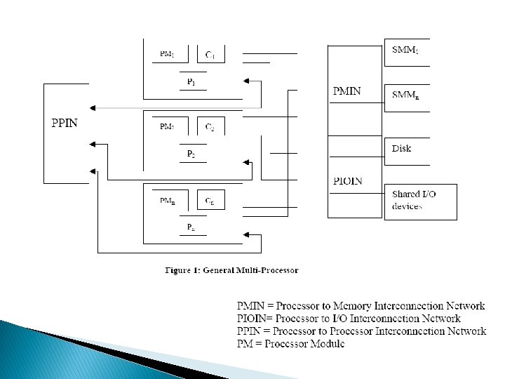
Introduction � � In multiprocessor systems, there are multiple processing elements, multiple I/O modules, and multiple memory modules. Each processor can access any of the memory modules and any of the I/O units. The connectivity between these is performed by interconnection networks. Thus, an interconnection network is used for exchanging data between two processors in a multistage network. Memory bottleneck is a basic shortcoming of Von Newman architecture. � In case of multiprocessor systems, the performance will be severely affected in case the data exchange between processors is delayed. The multiprocessor system has one global shared memory and each processor has a small local memory. The processors can access data from memory associated with another processor or from shared memory using an interconnection network. �

The interconnection networks are like customary network systems consisting of nodes and edges. � The nodes are switches having few input and few output (say n input and m output) lines. Depending upon the switch connection, the data is forwarded from input lines to output lines. � The interconnection network is placed between various devices in the multiprocessor network. � The architecture of a general multiprocessor is shown in Figure 1. In the multiprocessor systems, these are multiple processor modules (each processor module consists of a processing element, small sized local memory and cache memory), shared global memory and shared peripheral devices. �

NETWORK PROPERTIES � � Topology: It indicates how the nodes a network are organised. Network Diameter: It is the minimum distance between the farthest nodes in a network. The distance is measured in terms of number of distinct hops between any two nodes. Node degree: Number of edges connected with a node is called node degree. If the edge carries data from the node, it is called out degree and if this carries data into the node it is called in degree. Latency: It is the delay in transferring the message between two nodes.

NETWORK PROPERTIES � � Network throughput: It is an indicative measure of the message carrying capacity of a network. It is defined as the total number of messages the network can transfer per unit time. To estimate throughput, the capacity of the network and the messages number of actually carried by the network are calculated. Practically the throughput is only a fraction of its capacity. In interconnection network the traffic flow between nodes may be non uniform and it may be possible that a certain pair of nodes handles a disproportionately large amount of traffic. These are called “hot spot. ” The hot spot can behave as a bottleneck and can degrade the performance of the entire network.

NETWORK PROPERTIES � � � Data Routing Functions: The data routing functions are the functions which when executed establish the path between the source and the destination. Thus data routing operations are used for routing the data between various processors. The data routing network can be static or dynamic static network. Hardware Cost: It refers to the cost involved in the implementation of an interconnection network. It includes the cost of switches, arbiter unit, connectors, arbitration unit, and interface logic. Blocking and Non-Blocking network: In non-blocking networks the route from any free input node to any free output node can always be provided. Crossbar is an example of non-blocking network. In a blocking network simultaneous route establishment between a pair of nodes may not be possible. There may be situations where blocking can occur. Blocking refers to the situation where one switch is required to establish more than one connection simultaneously and end-to-end path cannot be established even if the input nodes and output nodes are free. The example of this is a blocking multistage network.

NETWORK PROPERTIES � � Static and Dynamic Interconnection Network: In a static network the connection between input and output nodes is fixed and cannot be changed. Static interconnection network cannot be reconfigured. The examples of this type of network are linear array, ring, tree, star. In dynamic network the interconnection pattern between inputs and outputs can be changed. The interconnection pattern can be reconfigured according to the program demands. Here, instead of fixed connections, the switches or arbiters are used. Examples of such networks are buses, crossbar switches, and multistage networks. The dynamic networks are normally used in shared memory(SM) multiprocessors.

NETWORK PROPERTIES � � Dimensionality of Interconnection Network: Dimensionality indicates the arrangement of nodes or processing elements in an interconnection network. In single dimensional or linear network, nodes are connected in a linear fashion; in two dimensional network the processing elements (PE’s) are arranged in a grid and in cube network they are arranged in a three dimensional network. Broadcast and Multicast : In the broadcast interconnection network, at one time one node transmits the data and all other nodes receive that data. Broadcast is one to all mapping. It is the implementation achieved by SIMD computer systems. Message passing multi-computers also have broadcast networks. In multicast network many nodes are simultaneously allowed to transmit the data and multiple nodes receive the data.

DESIGN ISSUES OF INTERCONNECTION NETWORK The following are the issues, which should be considered while designing an interconnection network. � Dimension and size of network: It should be decided how many PE’s are there in the network and what the dimensionality of the network is i. e. with how many neighburs, each processor is connected. � Symmetry of the network: It is important to consider whether the network is symmetric or not i. e. , whether all processors are connected with same number of processing elements, or the processing elements of corners or edges have different number of adjacent elements. � What is data communication strategy? Whether all processors are communicating with each other in one time unit synchronously or asynchronously on demand basis.

DESIGN ISSUES OF INTERCONNECTION NETWORK(Cont. . ) � � � Message Size: What is message size? How much data a processor can send in one time unit. Start up time: What is the time required to initiate the communication process. Data transfer time: How long does it take for a message to reach to another processor. Whether this time is a function of link distance between two processors or it depends upon the number of nodes coming in between.

VARIOUS INTERCONNECTION NETWORKS 1) Fully connected: This is the most powerful interconnection topology. In this each node is directly connected to all other nodes. The shortcoming of this network is that it requires too many connections.

VARIOUS INTERCONNECTION NETWORKS(Cont. . ) 2) Cross Bar: The crossbar network is the simplest interconnection network. It has a two dimensional grid of switches. It is a non-blocking network and provides connectivity between inputs and outputs and it is possible to join any of the inputs to any output. An N * M crossbar network is shown in the following Figure 3 (a) and switch connections are shown in Figure 3 (b). The crossbar network requires N 2 switches for N input and N output network.

VARIOUS INTERCONNECTION NETWORKS(Cont. . ) 3) Linear Array: This is a most fundamental interconnection pattern. In this processors are connected in a linear onedimensional array. The first and last processors are connected with one adjacent processor and the middle processing elements are connected with two adjacent processors. It is a one-dimensional interconnection network.

VARIOUS INTERCONNECTION NETWORKS(Cont. . ) 4) Mesh: It is a two dimensional network. In this all processing elements are arranged in a two dimensional grid. The processor in rows i and column j are denoted by Pei. The processors on the corner can communicate to two nearest neighbors i. e. PE 00 can communicate with PE 01 and PE 10. The processor on the boundary can communicate to 3 adjacent processing elements i. e. PE 01 can communicate with PE 00, PE 02 and PE 11 and internally placed processors can communicate with 4 adjacent processors i. e. PE 11 can communicate with PE 01, PE 10, PE 12, and PE 21

VARIOUS INTERCONNECTION NETWORKS(Cont. . ) � 5) Ring: This is a simple linear array where the end nodes are connected. It is equivalent to a mesh with wrap around connections. The data transfer in a ring is normally one direction. Thus, one drawback to this network is that some data transfer may require N/2 links to be traveled (like nodes 2 & 1) where N is the total number of nodes.

VARIOUS INTERCONNECTION NETWORKS(Cont. . ) 6) Torus: The mesh network with wrap around connections is called Tours Network.

VARIOUS INTERCONNECTION NETWORKS(Cont. . ) � 7) Tree interconnection network: In the tree interconnection network, processors are arranged in a complete binary tree pattern.

VARIOUS INTERCONNECTION NETWORKS(Cont. . ) 8) Fat tree: It is a modified version of the tree network. In this network the bandwidth of edge (or the connecting wire between nodes) increases towards the root. It is a more realistic simulation of the normal tree where branches get thicker towards root. It is the more popular as compared to tree structure, because practically the more traffic occurs towards the root as compared to leaves, thus if bandwidth remains the same the root will be a bottleneck causing more delay. In a tree this problem is avoided because of higher bandwidth.

VARIOUS INTERCONNECTION NETWORKS(Cont. . ) 9) Systolic Array: This interconnection network is a type of pipelined array architecture and it is designed for multidimensional flow of data. It is used for implementing fixed algorithms. Systolic array designed for performing matrix multiplication is shown below. All interior nodes have degree 6.

VARIOUS INTERCONNECTION NETWORKS(Cont. . ) 10) Cube: It is a 3 dimensional interconnection network. In this the PE’s are arranged in a cube structure.

VARIOUS INTERCONNECTION NETWORKS(Cont. . ) 11) Hyper Cube: A Hypercube interconnection network is an extension of cube network. Hypercube interconnection network for n ≥ 3, can be defined recursively as follows: � For n = 3, it cube network in which nodes are assigned number 0, 1, ……, 7 in binary. In other words, one of the nodes is assigned a label 000, another one as 001…. and the last node as 111. � Then any node can communicate with any other node if their labels differ in exactly one place, e. g. , the node with label 101 may communicate directly with 001, 000 and 111. � For n > 3, a hypercube can be defined recursively as follows: � Take two hypercubes of dimension (n – 1) each having (n – 1) bits labels as 00…. 0, …… 11…. . 1

VARIOUS INTERCONNECTION NETWORKS(Cont. . ) (Hyper Cube) � � Next join the two nodes having same labels each (n – 1) dimension hypercubes and join these nodes. Next prefix ‘ 1’ the labels of one of the (n – 1) dimensional hypercube and ‘ 0’ to the labels of the other hypercube. This completes the structure of n-dimensional hypercube. Direct connection is only between that pair of nodes which has a (solid) line connecting the two nodes in the pair. For n = 4 we draw 4 -dimensional hypercube as show in Figure 12:

VARIOUS INTERCONNECTION NETWORKS(Cont. . ) - Hyper Cube

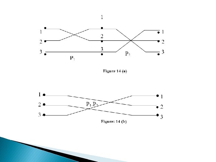
CONCEPT OF PERMUTATION NETWORK � � In permutation interconnection networks the information exchange requires data transfer from input set of nodes to output set of nodes and possible connections between edges are established by applying various permutations in available links. There are various networks where multiple paths from source to destination are possible. For finding out what the possible routes in such networks are the study of the permutation concept is a must. Let us look at the basic concepts of permutation with respect to interconnection network. Let us say the network has set of n input nodes and n output nodes. Permutation P for a network of 5 nodes (i. e. , n = 5) is written as follows:

� It means node connections are 1↔ 5, 2↔ 4, 3↔ 1, 4↔ 3, 5↔ 2. The connections are shown in the Figure 13. � The other permutation of the same set of nodes may be � � Which means connections are: 1↔ 2, 2↔ 3, 3↔ 5, 4↔ 1, and 5↔ 4

� Similarly, other permutations are also possible. The Set of all permutations of a 3 -node network will be Connection, indicates connection from node 1 to node 1, node 2 to node 2, and node 3 to node 3, hence it has no meaning, so it is dropped. � In these examples, only one set of links exist between input and output nodes and means it is a single stage network. It may be possible that there exist multiple links between input and output (i. e. multistage network). Permutation of all these in a multistage network are called permutation group and these are represented by a cycle. � e. g. permutation consists of nodes 1, 2, 3 and another group consists of nodes 4, 5 and connections are 1→ 2, 2→ 3, 3→ 1, and 4→ 5. Here group (1, 2, 3) has period 3 and (4, 5) has period 2, collectively these groups has periodicity 3× 2=6.

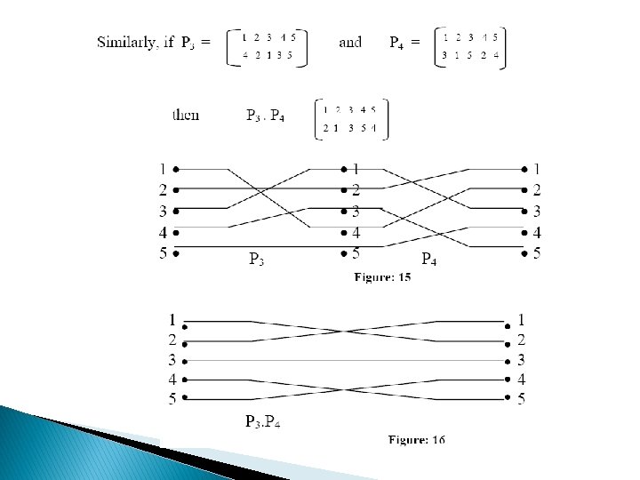
� � � Interconnection from all the possible input nodes to all the output nodes forms the permutation group. The permutations can be combined. This is called composition operation. In composition operation two or more permutations are applied in sequence, e. g. if P 1 and P 2 are two permutations defined as follows: The composition of P 1 and P 2 will be

� 1) There are few permutations of special significance in interconnection network. These permutations are provided by hardware. Now, let us discuss these permutations in detail. Perfect Shuffle Permutation: This was suggested by Harold Stone (1971). Consider N objects each represented by n bit number say Xn-1, Xn-2, X 0 (N is chosen such that N = 2 n. ) The perfect shuffle of these N objects is expressed as That, means perfect shuffle is obtained by rotating the address by 1 bit left. e. g. shuffle of 8 objects is shown as

2) Butterfly permutation: This permutation is obtained by interchanging the most significant bit in address with least significant bit.

3) Clos network: This network was developed by Clos (1953). It is a non-blocking network and provides full connectivity like crossbar network but it requires significantly less number of switches. The organization of Clos network is shown in Figure 19:

� � � � Consider an I input and O output network Number N is chosen such that (I= n. x) and (O=p. y). In Clos network input stage will consist of X switches each having n input lines and z output lines. The last stage will consist of Y switches each having m input lines and p output lines and the middle stage will consist of z crossbar switches, each of size X × Y. To utilize all inputs the value of Z is kept greater than or equal to n and p. The connection between various stages is made as follows: all outputs of 1 st crossbar switch of first stage are joined with 1 st input of all switches of middle stage. (i. e. , 1 st output of first page with 1 st middle stage, 2 nd output of first stage with 1 st input of second switch of middle stage and so on…) The outputs of second switch of first stage. Stage are joined with 2 nd input of various switches of second stage (i. e. , 1 st output of second switch of 1 st stage is joined with 2 input of 1 st switch of middle stage and 2 nd output of 2 nd switch of 1 st stage is joined with 2 nd input of 2 nd switch of middle stage and so on… Similar connections are made between middle stage and output stage (i. e. outputs of 1 st switch of middle stage are connected with 1 st input of various switches of third stage. Permutation matrix of P in the above example the matrix entries will be n

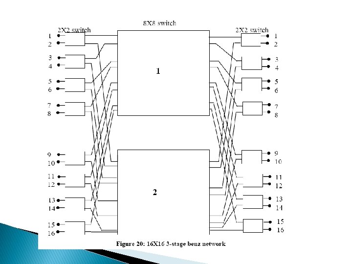
4) Bens Network: It is a non-blocking network. It is a special type of Clos network where first and last stage consists of 2× 2 switches (for n input and m output network it will have n/2 switches of 2 × 2 order and the last stage will have m/2 switch of 2× 2 order the middle stage will have two n/2 Χ m/2 switches. Numbers n and m are assumed to be the power of 2. Thus, for 16× 16 3 -stage Bens network first stage and third stage will consist of 8 (2× 2) switches and middle stage will consist of 2 switches of size (8× 8). The connection of crossbar will be as follows:

� � The switches of various stages provide complete connectivity. Thus by properly configuring the switch any input can be passed to any output. Consider a Clos network with 3 stages and 3× 3 switches in each stage.

� � The implementation of this above permutation is shown in Figure 20. This permutation can be represented by the following matrix also, Elements of Parallel Computing and Architecture

� � � The upper input of all first stage switches will be connected with respective inputs of 1 st middle stage switch, and lower input of all first stage switches will be connected with respective inputs of 2 nd switch. Similarly, all outputs of 1 st switch of middle stage will be connected as upper input of switches at third stage. In Benz network to reduce the complexity the middle stage switches can recursively be broken into N/4 × N/4 (then N/8 × M/8), till switch size becomes 2× 2. The connection in a 2× 2 switch will either be straight, exchange, lower broadcast or upper broadcast as shown in the Figure.

� The 8× 8 Benz network with all switches replaced by a 2× 2 is shown in Figure 23(a):

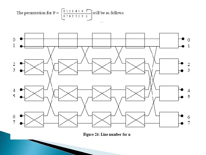
� The Bens network connection for permutation

The End