Multiprocessors Interconnection Networks An interconnection network could be

Multiprocessors Interconnection Networks An interconnection network could be either static or dynamic. Connections in a static network are fixed links, while connections in a dynamic network are established on the fly as needed. A topology-based taxonomy for interconnection networks : Static networks : one-dimension (1 D), two-dimension (2 D), Hypercube (HC). Switch-based dynamic networks can be classified according to the structure of the interconnection network as single-stage (SS), multistage (MS), or crossbar networks

Bus-Based Dynamic Interconnection Networks 1 - Single Bus Systems In its general form, such a system consists of N processors, each having its own cache, connected by a shared bus. The use of local caches reduces the processor–memory traffic. All processors communicate with a single shared memory. The actual size is determined by the traffic per processor and the bus bandwidth. The single bus network complexity, measured in terms of the number of buses used, is O(1), while the time complexity, measured in terms of the amount of input to output delay is O(N).

2 - Multiple Bus Systems A multiple bus multiprocessor system uses several parallel buses to interconnect multiple processors and multiple memory modules. A number of connection schemes are possible in this case. (a) -MBFBMC: multiple bus with full bus–memory connection (b) -MBSBMC: multiple bus with single bus memory connection (c) -MBPBMC: multiple bus with partial bus–memory connection (d) -MBCBMC: multiple bus with class-based memory connection. The multiple bus with full bus–memory connection has all memory modules connected to all buses. The multiple bus with single bus– memory connection has each memory module connected to a specific bus. The multiple bus with partial bus–memory connection has each memory module connected to a subset of buses. The multiple bus with class-based memory connection has memory modules grouped into classes whereby each class is connected to a specific subset of buses. A class is just an arbitrary collection of memory modules. Illustrations of these connection schemes for the case of N = 6 processors, M = 4 memory modules, and B = 4 buses as below:
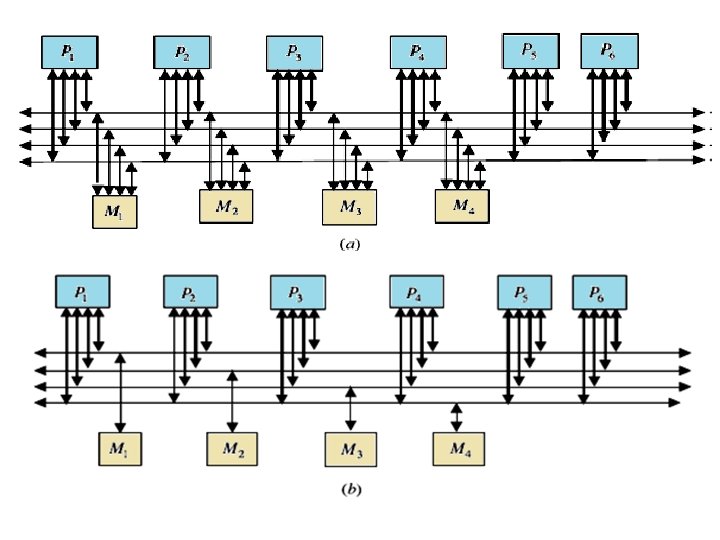

One can characterize those connections using the number of connections required and the load on each bus as shown in Table. In this table, k represents the number of classes; g represents the number of buses per group, and Mj represents the number of memory modules in class j. TABLE of Characteristics of Multiple Bus Architectures multiple bus multiprocessor organization offers a number of desirable features such as high reliability and ease of incremental growth. A single bus failure will leave (B-1) distinct fault-free paths between the processors and the memory modules. On the other hand, when the number of buses is less than the number of memory modules (or the number of processors), bus contention is expected to increase.

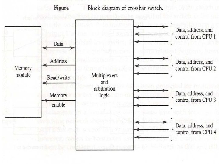
Switch-Based Interconnection Networks In this type of network, connections among processors and memory modules are made using simple switches. Three basic interconnection topologies exist: crossbar, single-stage, and multistage. 1 - Crossbar Networks 2 - Single-Stage Networks 3 - Multistage Networks 1 - Crossbar Networks: While the single bus can provide only a single connection, the crossbar can provide simultaneous connections among all its inputs and all its outputs. The crossbar contains a switching element (SE) at the intersection of any two lines extended horizontally or vertically inside the switch. For example the 8 x 8 crossbar network an SE (also called a cross-point) is provided at each of the 64 SEs or (intersection points) and the message delay to traverse from the input to the output is constant, regardless of which input/output are communicating.
. In")
The two possible settings of an SE in the crossbar (straight and diagonal). In general for an Nx. N crossbar, the network complexity, measured in terms of the number of switching points, is O(N 2) while the time complexity, measured in terms of the input to output delay, is O(1). An 8 x 8 crossbar network (a) straight switch setting; (b) diagonal switch setting

2 - Single-Stage Networks The simplest switching element that can be used is the 2 x 2 switching element (SE). With four possible settings A well-known connection pattern for interconnecting the inputs(source) and the outputs (destination)of a single-stage network is the Shuffle– Exchange. Two operations are used. These can be defined using an m bit -wise address pattern of the inputs, pm-1 pm-2. . . p 1 p 0, as follows: If the number of inputs, for example, processors, in a single-stage IN is N and the number of outputs, for example, memories, is N, the number of SEs in a stage is N/2. The maximum length of a path from an input to an output in the network, measured by the number of SEs along the path, is log 2 N. The network complexity of the single-stage interconnection network is O(N) and the time complexity is O(N).
")
Example In an 8 -input single stage Shuffle–Exchange if the source is 0 (000) and the destination is 6 (110), then the following is the required sequence of Shuffle/ Exchange operations and circulation of data: In addition to the shuffle and the exchange functions, there exist other interconnection patterns. Among these are the Cube and the Plus. Minus 2 i(PM 2 I) networks. The Cube Network Consider a 3 -bit address (N = 8), we have C 2(6) = 2, C 1(7) = 5 C 0(4) = 5.
 Network The PM 2 I network consists")
The Plus–Minus 2 i (PM 2 I) Network The PM 2 I network consists of 2 k interconnection functions defined as below: For example, consider the case N = 8, PM 2+1(4) =4 + 21 mod 8 = 6. The PM 2 I network for N =8 (a), PM 2+0 for N = 8; (b) PM 2+1 for N =8; (c) PM 2+2 for N = 8.

The Butterfly Function The interconnection pattern used in the butterfly network is defined as follows: Consider a 3 -bit address (N =8), the following is the butterfly mapping:
")
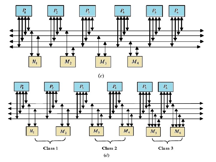
Multistage Networks The most undesirable single bus limitation that Multistage interconnection networks (MINs ) is set to improve is the availability of only one single path between the processors and the memory modules. Such MINs provide a number of simultaneous paths between the processors and the memory modules. A general MIN consists of a number of stages each consisting of a set of 2 x 2 switching elements. Stages are connected to each other using Interstage Connection (ISC) Pattern. These patterns may follow any of the routing functions such as Shuffle–Exchange, Butterfly, Cube, and so on. The settings of the SEs give a number of paths can be established simultaneously. For example, the figure below shows how three simultaneous paths connecting the three pairs of input/output 000 → 101, 101→ 011, and 110→ 010 can be established. It should be noted that the interconnection pattern among stages follows the shuffle operation. This network is known as the Shuffle–Exchange network (SEN). as An example 8 x 8 (SEN).

The Banyan Network The memory modules, is N, the number of MIN stages is log 2 N and the number of SEs per stage is N/2, and hence the network complexity, measured in terms of the total number of SEs is O(N x log 2 N). The time complexity, measured by the number of SEs along the path from input to output, is O(log 2 N). For example, in a 16 x 16 MIN, the length of the path from input to output is 4. The total number of SEs in the network is usually taken as a measure for the total area of the network. The total area of a 16 x 16 MIN is 32 SEs.
 Number of Switches per")
The Omega Network Number of Stages = (Log 2 n) Number of Switches per Stage = (n/2), Total Switches = (n/2)Log 2 n A size N omega network consists of n (n=log 2 N single-stage) Shuffle– Exchange networks. Each stage consists of a column of N=2, two-input switching elements whose input is a shuffle connection

A commonly used multistage connection network is the omega network. This network consists of log p stages, where p is the number of inputs (processing nodes) and also the number of outputs (memory banks). Each stage of the omega network consists of an interconnection pattern that connects p inputs and p outputs; a link exists between input i and output j if the following is true:

Equation 6. 1 represents a left-rotation operation on the binary representation of i to obtain j. This interconnection pattern is called a perfect shuffle. Figure below shows a perfect shuffle interconnection pattern for eight inputs and outputs. At each stage of an omega network, a perfect shuffle interconnection pattern feeds into a set of p/2 switches or switching nodes. It should be noted that the interconnection pattern among stages follows the shuffle operation.

CPU 011 read From 110 Message Format • • Module It tell which memory to use. Address It specifies an address within a module Opcode Gives the operation, READ or WRITE Value Contain an operand.

Blockage in Multistage Interconnection Networks A number of classification criteria exist for MINs. Among these criteria is the criterion of blockage. According to this criterion, MINs are classified as follows. Blocking Networks the concept of blocking network is that not all possible here to make the input-output connections at the same time as one path might block another. Examples of blocking networks include Omega, Banyan, Shuffle–Exchange, the Data Manipulator, Flip, N cube and Baseline. Rearrangeable Networks: Re-arrangeable networks are characterized by the property that it is always possible to rearrange already established connections in order to make allowance for other connections to be established simultaneously. An example is Benes network which support synchronous data permutation and a synchronous inter-processor communication. Non-blocking Networks A non –blocking network is the network which can handle all possible connections without blocking.

In the presence of a connection between input 101 and output 011, a connection between input 100 and output 001 is not possible. This is because the connection 101 to 011 uses the upper output of the third switch from the top in the first stage. This same output will be needed by the requested connection 100 to 001. This contention will lead to the inability to satisfy the connection 100 to 001, that is, blocking. Notice however that while connection 101 to 011 is established, the arrival of a request for a connection such as 100 to 110 can be satisfied.

In the presence of a connection between input 101 and output 011, a connection between input 100 and output 001 is not possible. This is because the connection 101 to 011 uses the upper output of the third switch from the top in the first stage. This same output will be needed by the requested connection 100 to 001. This contention will lead to the inability to satisfy the connection 100 to 001, that is, blocking. Notice however that while connection 101 to 011 is established, the arrival of a request for a connection such as 100 to 110 can be satisfied.

an example 8 x 8 Benes network. Two simultaneous connections are shown established in the network. These are 110→ 100 and 010→ 110. In the presence of the connection 110→ 100, it will not be possible to establish the connection 101→ 001 unless the connection 110→ 100 is rearranged as shown in part (b) of the figure.

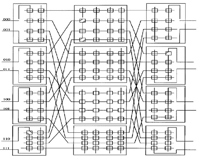
Non-blocking Networks The Clos is a well-known example of non-blocking networks. It consists of r 1 n 1 x m input crossbar switches (r 1 is the number of input crossbars, m xn 1 is the size of each input crossbar), mr 1 x r 2 middle crossbar switches (m is the number of middle crossbars, and r 1 x r 2 is the size of each middle crossbar), r 2 m x n 2 output crossbar switches (r 2 is the number of output crossbars and m x n 2 is the size of each output crossbar). The Clos network is not blocking if the following inequality is satisfied m ≥ n 1+ n 2 – 1 A three-stage Clos network is shown in Figure below. The network has the following parameters: r 1 = 4, n 1 = 2, m = 4, r 2 = 4, and n 2 = 2. The reader is encouraged to ascertain the non-blocking feature of the network shown in Figure below by working out some example simultaneous connections. For example show that in the presence of a connection such as 110 to 010, any other connection will be possible.

Mesh-Connected Illiac Networks Here in mesh network nodes are arranged as a q-dimensional lattice. The neighboring nodes are only allowed to communicate the data in one step i. e. , each PEi is allowed to send the data to any one of PE(i+1) , PE (i-1), Pe(i+r) and PE(i-r) where r= square root N( in case of Iliac r=8). In a periodic mesh, nodes on the edge of the mesh have wrap-around connections to nodes on the other side this is also called a to roidal mesh. Mesh Metrics For a q-dimensional non-periodic lattice with kq nodes: • Network connectivity = q • Network diameter = q(k-1) • Network narrowness = k/2 • Bisection width = kq-1 • Expansion Increment = kq-1 • Edges per node = 2 q Thus we observe the output of ISk is connected to inputs of OSj where j = k-1, K+1, k-r, k+r as shown in figure.

Similarly the OSj gets input from ISk for K= j-1, j+1, j-r, j+r. The topology is formerly described by the four routing functions: • R+1(i)= (i+1) mod N => (0, 1, 2…, 14, 15) • R-1(i)= (i-1) mod N => (15, 14, …, 2, 1, 0) • R+r(i)= (i+r) mod N => (0, 4, 8, 12)(1, 5, 9, 13)(2, 6, 10, 14)(3, 7, 11, 15) • R-r(i)= (i-r) mod N => (15, 11, 7, 3)(14, 10, 6, 2)(13, 9, 5, 1)(12, 8, 4, 0) The figure given below show each PEi is connected to its four nearest neighbors in the mesh network. It is same as that used for IILiac – IV except that w had reduced it for N=16 and r=4. The index are calculated as module N. An n-dimensional mesh can be defined as an interconnection structure that has K 0 x K 1 x……. . Kn-1 nodes. where n is the number of dimensions of the network Ki is the radix of dimension i. shows an example of a 3 x 3 x 2 mesh network.
 is connected to its neighbors at")
A node whose position is (i, j, k) is connected to its neighbors at dimensions i± 1, j± 1, and k± 1. Mesh architecture with wrap around connections forms a torus. A number of routing mechanisms have been used to route messages around meshes. One such routing mechanism is known as the dimension-ordering routing. Using this technique, a message is routed in one given dimension at a time, arriving at the proper coordinate in each dimension before proceeding to the next dimension. A 3 x 3 x 2 mesh network Consider, for example, a 3 D mesh. Since each node is represented by its position (i, j, k), then messages are first sent along the i dimension, then along the j dimension, and finally along the k dimension. At most two turns will be allowed and these turns will be from i to j and then from j to k. In Figure we show the route of a message sent from node S at position (0, 0, 0) to node D at position (2, 1, 1). Other routing mechanisms in meshes have been proposed. It should be noted that for a mesh interconnection network with N nodes, the longest distance traveled between any two arbitrary nodes is O(√N).

Permutation Networks Thus the permutation cycle according to routing function will be as follows: Horizontally, all PEs of all rows form a linear circular list as governed by the following two permutations, each with a single cycle of order N. The permutation cycles (a b c) (d e) stands for permutation a->b, b->c, c->a and d->e, e->d in a circular fashion with each pair of parentheses. R+1 = (0 1 2 …. N-1) R– 1 = (N-1 …. . 2 1 0). Similarly we have vertical permutation also and now by combining the two permutation each with four cycles of order four each the shift distance for example for a network of N = 16 and r = square root(16) = 4, is given as follows: R +4 = (0 4 8 12)(1 5 9 13)(2 6 10 14)(3 7 11 15) R – 4 = (12 8 4 0)(13 9 5 1)(14 10 6 2)(15 11 7 3) Mesh Redrawn
 interconnection networks are characterized by having fixed paths, unidirectional")
Static Interconnection Networks Static (fixed) interconnection networks are characterized by having fixed paths, unidirectional or bidirectional, between processors. Two types of static networks can be identified. These are completely connected networks (CCNs) and limited connection networks (LCNs). a) Completely Connected Networks In a completely connected network (CCN) each node is connected to all other nodes in the network. Completely connected networks guarantee fast delivery of messages from any source node to any destination node (only one link has to be traversed). q Routing of messages between nodes becomes a straightforward task. q Expensive in terms of the number of links needed for their construction (more apparent for higher values of N). q The number of links is given by N(N - 1)/2. The delay complexity of CCNs, measured in terms of the number of links traversed as messages are routed from any source to any destination is constant, that is, O(1). An example having N = 6 nodes is shown below:
 do not provide a direct link")
b- Limited Connection Networks Limited connection networks (LCNs) do not provide a direct link from every node to every other node in the network. Instead, communications between some nodes have to be routed through other nodes in the network. The length of the path between nodes, measured in terms of the number of links that have to be traversed, is expected to be longer compared to the case of CCNs. Two other conditions seem to have been imposed by the existence of limited interconnectivity in LCNs. These are: 1 - the need for a pattern of interconnection among nodes 2 -the need for a mechanism for routing messages around the network until they reach their destinations.

A number of regular interconnection patterns have evolved over the years for LCNs. These patterns include: One dimensional topologies (a linear array network; ( simple routing mechanism but slow. ) Various 2 -D topologies : (b)ring (loop) networks; (c) two-dimensional arrays (mesh) -(nearest-neighbor mesh); (d) tree networks; star ; Systolic Array 3 -D topologies (Completely connected chordal ring ; Chordal ring ; 3 cube
 in a binary tree system having k")
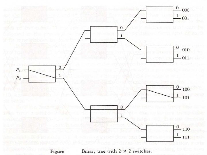
Tree Network The number of nodes (processors) in a binary tree system having k levels can be calculated as: Notice that the maximum depth of a binary tree system is, where N is the number of nodes (processors) in the network. Therefore, the network complexity is O(2 k) and the time complexity is O( log 2 N). Cube-Connected Networks Cube-connected networks are patterned after the n-cube structure. An ncube (hypercube of order n) is defined as an undirected graph having 2 n vertices labeled 0 to 2 n - 1 such that there is an edge between a given pair of vertices if and only if the binary representation of their addresses differs by one and only one bit. A 4 -cube is shown in Figure. In an n-cube, each node has a degree n. The degree of a node is defined as the number of links incident on the node. The maximum number of links a message has to traverse in order to reach its destination in an n-cube containing N = 2 n nodes is log 2 N = n links.
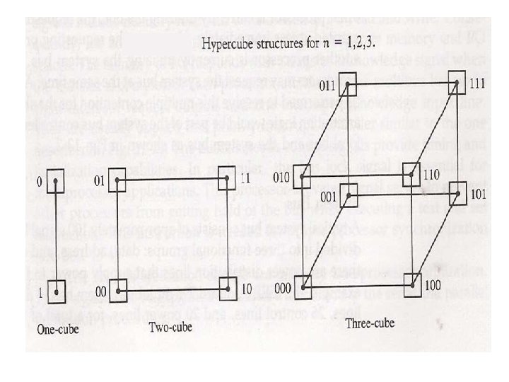

In an n-cube, each processor has communication links to n other processors. The route of a message originating at node i and destined for node j can be found by XOR-ing the binary address representation of i and j. If the XOR-ing operation results in a 1 in a given bit position, then the message has to be sent along the link that spans the corresponding dimension. For example, if a message is sent from source (S) node 0101 to destination (D) node 1011, then the XOR operation results in 1110. That will mean that the message will be sent only along dimensions 2, 3, and 4 (counting from right to left) in order to arrive at the destination. The order in which the message traverses the three dimensions is not important.

Torus architecture is also one of popular network topology it is extension of the mesh by having wraparound connections Figure below is a 2 D Torus This architecture of torus is a symmetric topology unlike mesh which is not. The wraparound connections reduce the torus diameter and at the same time restore the symmetry. It can be o 1 -D torus 2 -D torus 3 -D torus The torus topology is used in Cray T 3 E We can have further higher dimension circuits for example 3 -cube connected cycle. A D- dimension W-wide hypercube contains W nodes in each dimension and there is a connection to a node in each dimension. The mesh and the cube architecture actually 2 -D and 3 -D hypercube respectively. The below figure we have hypercube with dimension 4.

Routing Algorithm for Omega Network To understand this routing algorithm, consider the 1 st stage of the Omega network to the right. n 1 All four 1 st stage switches send their upper outputs to switches E and G, and their lower outputs to switches F and H. n 2 3 4 Switches E and G both send their outputs to switches I and J; their data can only reach the network outputs of 0, 1, 2, and 3. n 0 5 6 7 A E I B F J C G K D H L Similarly, data from switches F and H can only reach network It should be noted that the interconnection outputs 4, 5, 6, and 7. n pattern among stages follows the shuffle operation. 0 1 2 3 4 5 6 7
 (100) set so that its")
BLOCKED Each 1 st stage switch must be (111) (100) set so that its upper output has a 0 0 E I (111) A destination with binary value 000, 1 1 001, 010, or 011, i. e. having 0 in 2 2 B F J the first bit position of its 3 3 destination. 4 4 n Similarly, the lower output of C G K 5 each 1 st stage switch must have a 1 5 6 6 in the first bit position of its D H L destination to reach outputs 100, 7 7 101, 110, or 111. n For example, if network input 0 has to establish a connection with network output 7 (111), then the uppermost 1 st stage switch must set itself to exchange. n If two inputs to a 1 st stage switch have the same value in the first bit position, the Omega network cannot realize this permutation. n For example, if network input 0 has network output 4 and network input 1 has network output 7 as their destinations, then switch A is blocked since both 4 (100) and 7 (111) have bit 1 in their first bit position. n

Similarly, the 2 nd stage switch sends its upper output to switches I or K, which connect to outputs 0 (000), 1 (001), 4 (100), and 5 (101). n The lower outputs can reach switches J or L, which can access outputs 2, 3, 6, and 7 (010, 011, 110, and 111). n For the second stage, the 2 nd bit of the destination determines the setting of the switch. n Similarly, the least significant bit of the destination determines the setting of the switches in the 3 rd stage. n Since the 3 rd stage outputs are the outputs of the network, the last stage cannot block a permutation that has been routed successfully by the previous stages. 0 1 A E I B F J 4 5 C G K 4 5 6 7 D H L 6 7 2 3 n

Successful Omega Routing Scheme 0 111 1 011 000 001 0 1 000 2 001 3 110 4 000 5 101 111 010 7 100 2 3 101 010 6 011 110 100 010 101 4 5 100 111 6 110 7

Unsuccessful Omega Routing 0 100 1 000 BLOCK 0 1 001 2 101 3 011 4 111 5 001 100 3 111 010 7 110 100 BLOCK 010 6 2 101 110 4 5 101 111 6 110 7

Conclusion Interconnection networks play a central role in determining the overall performance of a multiprocessor system. And if the interconnection network cannot minimize its message latency for a particular application, then processors will frequently be forced to wait for data to arrive. n The table below gives some qualitative comparisons between the various types of interconnection configurations. l Property Bus Crossbar Multistage Speed Low High Cost Low High Moderate Reliability Low High Configurability High Low Moderate Complexity Low High Moderate

45
- Slides: 45