GRADING POLICY Quizees Midterm exam Final exam Grade

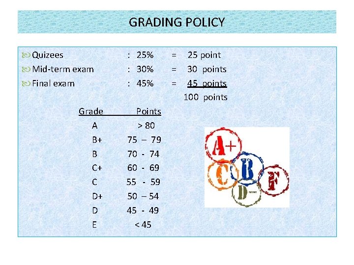
GRADING POLICY Quizees Mid-term exam Final exam Grade A B+ B C+ C D+ D E : 25% : 30% : 45% Points > 80 75 – 79 70 - 74 60 - 69 55 - 59 50 – 54 45 - 49 < 45 = = = 25 point 30 points 45 points 100 points

What is statistics The mathematics of the collection, organization, and interpretation of numerical data, especially the analysis of population characteristics by inference from sampling Why statistics • Need to make quantified statements about a phenomenon we are interested in • …Therefore we collect samples as proxies of the greater population of individuals or items that make up the phenomenon we are interested in • Anything can be expressed in statistics Aims of the course • Introduction to basic statistics • Learn to use analysis tools in EXCEL • Make you an intelligent user of data and statistics

We will bypass much of the mathematics, instead emphasizing the understanding of underlying principles Types of statistics 1. Descriptive statistics Quantitative methods of organizing, summarizing, and presenting data in an informative way (numerically, graphically) Describe the overall characteristics of a sample Transform raw data into more easily understood forms 2. Inferential statistics The branch of statistics used to make inferences about a larger population based on the data collected from a sample Make prediction

• Parametric statistics • Non parametric statistics • Primary data • Secondary data • Quantitative data • Qualitative data • Discrete data • Continuous data

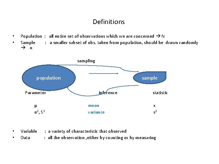
Definitions • • Population : all entire set of observations which we are concerned N Sample : a smaller subset of obs. taken from population, should be drawn randomly n sampling population Parameter µ σ2 , S 2 • • Variable Data sample inference mean variance statistic x s 2 : a variety of characteristic that observed : all the observation , either by counting or by measuring

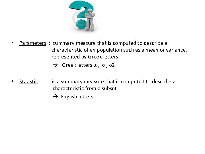
• Parameters : summary measure that is computed to describe a characteristic of an population such as a mean or variance, represented by Greek letters μ , σ2 • Statistic : is a summary measure that is computed to describe a characteristic from a subset English letters

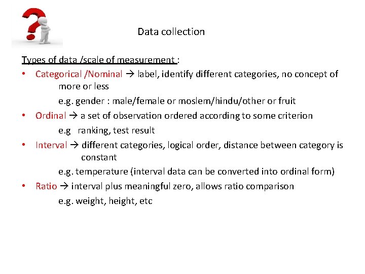
Data collection Types of data /scale of measurement : • Categorical /Nominal label, identify different categories, no concept of more or less e. g. gender : male/female or moslem/hindu/other or fruit • Ordinal a set of observation ordered according to some criterion e. g ranking, test result • Interval different categories, logical order, distance between category is constant e. g. temperature (interval data can be converted into ordinal form) • Ratio interval plus meaningful zero, allows ratio comparison e. g. weight, height, etc

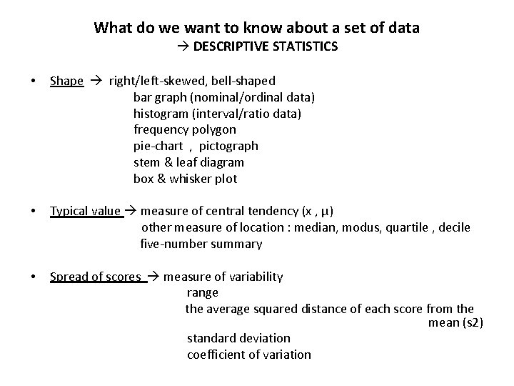
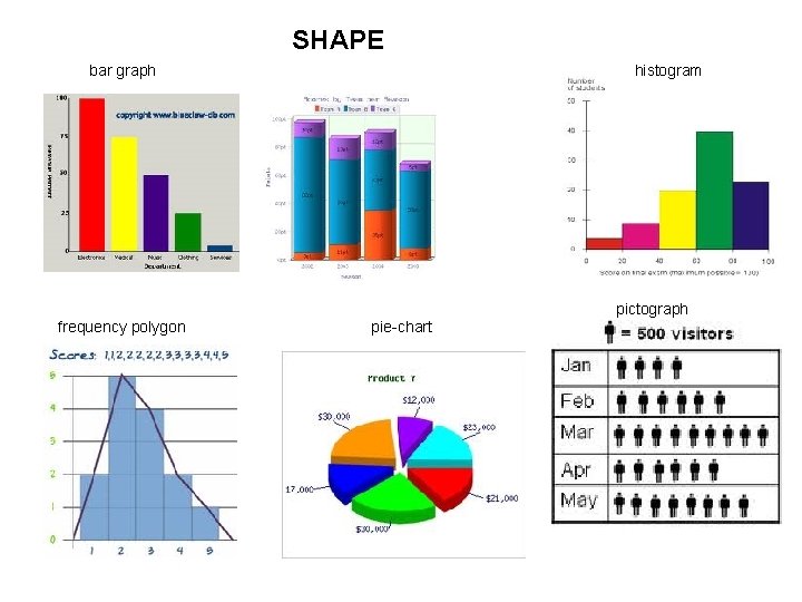
What do we want to know about a set of data DESCRIPTIVE STATISTICS • Shape right/left-skewed, bell-shaped bar graph (nominal/ordinal data) histogram (interval/ratio data) frequency polygon pie-chart , pictograph stem & leaf diagram box & whisker plot • Typical value measure of central tendency (x , μ) other measure of location : median, modus, quartile , decile five-number summary • Spread of scores measure of variability range the average squared distance of each score from the mean (s 2) standard deviation coefficient of variation

SHAPE bar graph histogram pictograph frequency polygon pie-chart

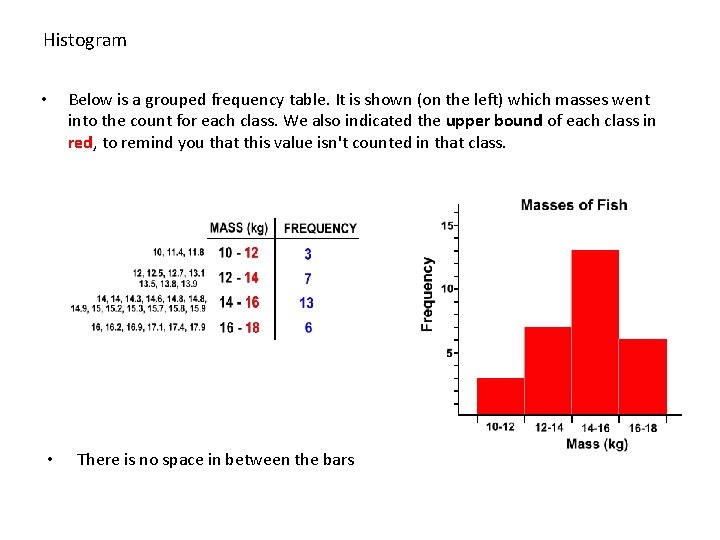
Histogram • • Below is a grouped frequency table. It is shown (on the left) which masses went into the count for each class. We also indicated the upper bound of each class in red, to remind you that this value isn't counted in that class. There is no space in between the bars

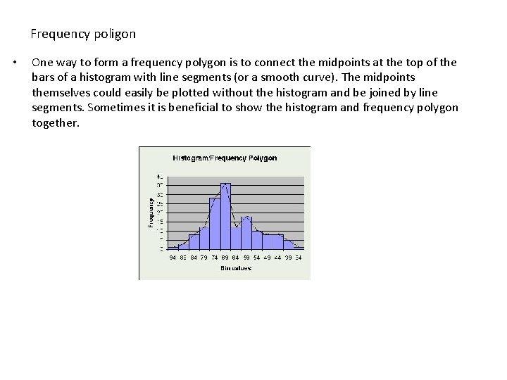
Frequency poligon • One way to form a frequency polygon is to connect the midpoints at the top of the bars of a histogram with line segments (or a smooth curve). The midpoints themselves could easily be plotted without the histogram and be joined by line segments. Sometimes it is beneficial to show the histogram and frequency polygon together.

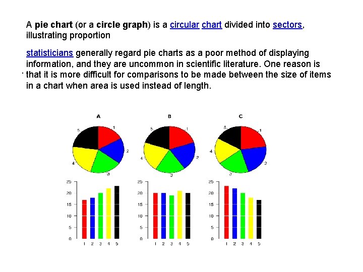
A pie chart (or a circle graph) is a circular chart divided into sectors, illustrating proportion statisticians generally regard pie charts as a poor method of displaying information, and they are uncommon in scientific literature. One reason is. that it is more difficult for comparisons to be made between the size of items in a chart when area is used instead of length.

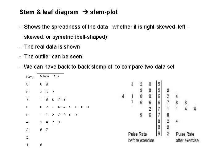
Stem & leaf diagram stem-plot - Shows the spreadness of the data whether it is right-skewed, left – skewed, or symetric (bell-shaped) - The real data is shown - The outlier can be seen - We can have back-to-back stemplot to compare two data set

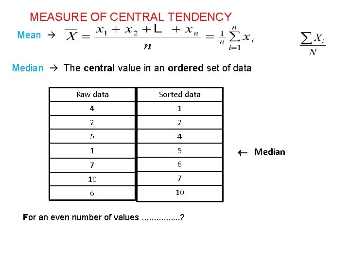
MEASURE OF CENTRAL TENDENCY Mean Median The central value in an ordered set of data Raw data Sorted data 4 1 2 2 5 4 1 5 7 6 10 For an even number of values. . . . ? Median

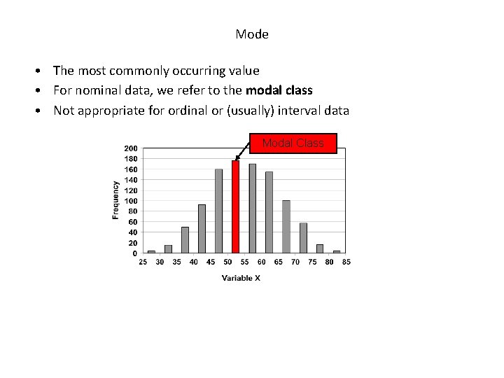
Mode • The most commonly occurring value • For nominal data, we refer to the modal class • Not appropriate for ordinal or (usually) interval data Modal Class

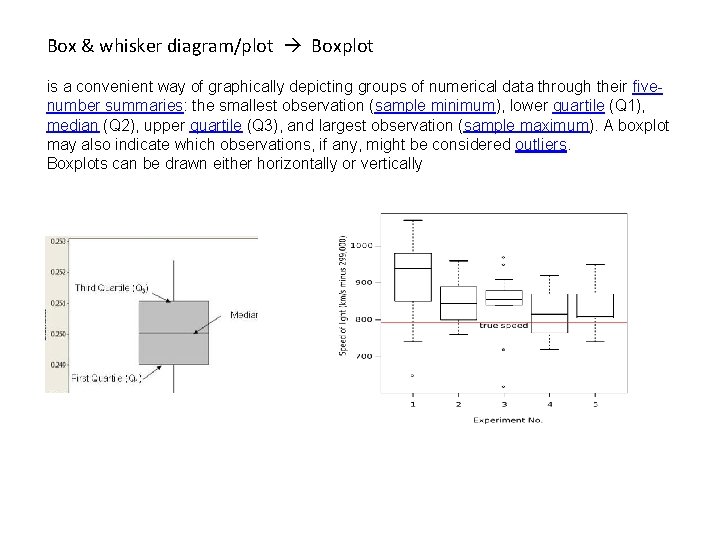
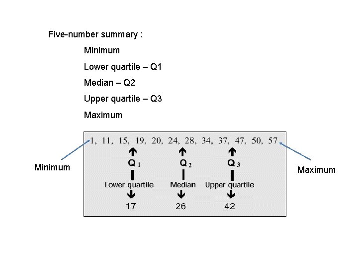
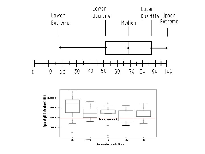
Box & whisker diagram/plot Boxplot is a convenient way of graphically depicting groups of numerical data through their fivenumber summaries: the smallest observation (sample minimum), lower quartile (Q 1), median (Q 2), upper quartile (Q 3), and largest observation (sample maximum). A boxplot may also indicate which observations, if any, might be considered outliers. Boxplots can be drawn either horizontally or vertically

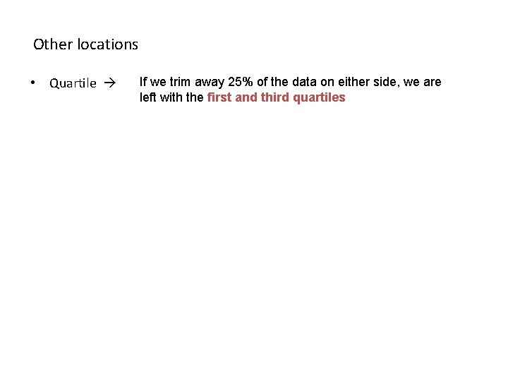
Other locations • Quartile If we trim away 25% of the data on either side, we are left with the first and third quartiles

Five-number summary : Minimum Lower quartile – Q 1 Median – Q 2 Upper quartile – Q 3 Maximum Minimum Maximum

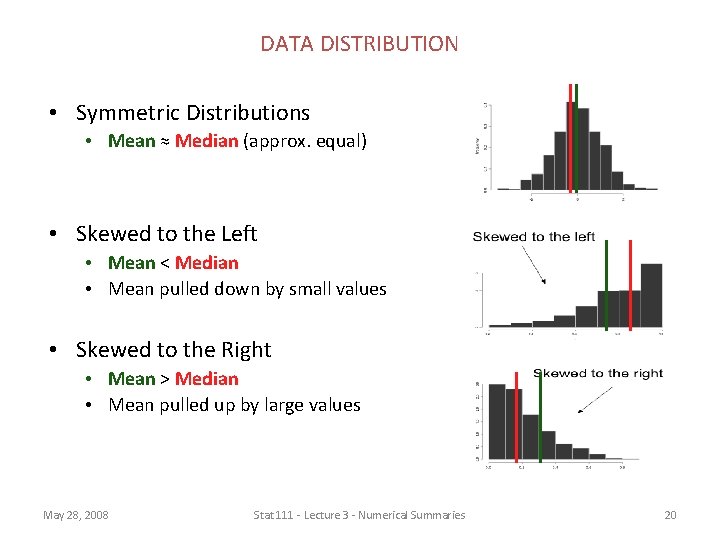
DATA DISTRIBUTION • Symmetric Distributions • Mean ≈ Median (approx. equal) • Skewed to the Left • Mean < Median • Mean pulled down by small values • Skewed to the Right • Mean > Median • Mean pulled up by large values May 28, 2008 Stat 111 - Lecture 3 - Numerical Summaries 20

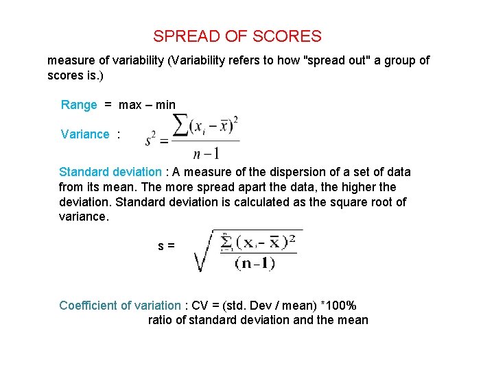
SPREAD OF SCORES measure of variability (Variability refers to how "spread out" a group of scores is. ) Range = max – min Variance : Standard deviation : A measure of the dispersion of a set of data from its mean. The more spread apart the data, the higher the deviation. Standard deviation is calculated as the square root of variance. s= Coefficient of variation : CV = (std. Dev / mean) *100% ratio of standard deviation and the mean

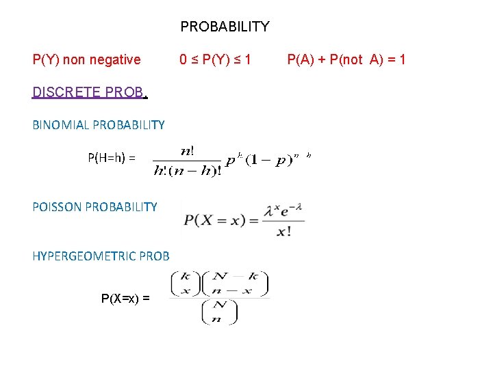
PROBABILITY P(Y) non negative DISCRETE PROB. BINOMIAL PROBABILITY P(H=h) = POISSON PROBABILITY HYPERGEOMETRIC PROB P(X=x) = 0 ≤ P(Y) ≤ 1 P(A) + P(not A) = 1

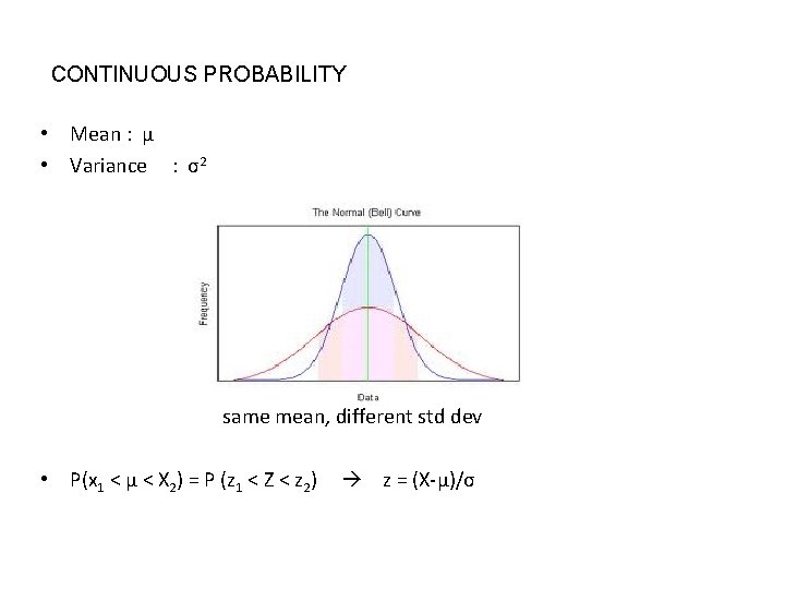
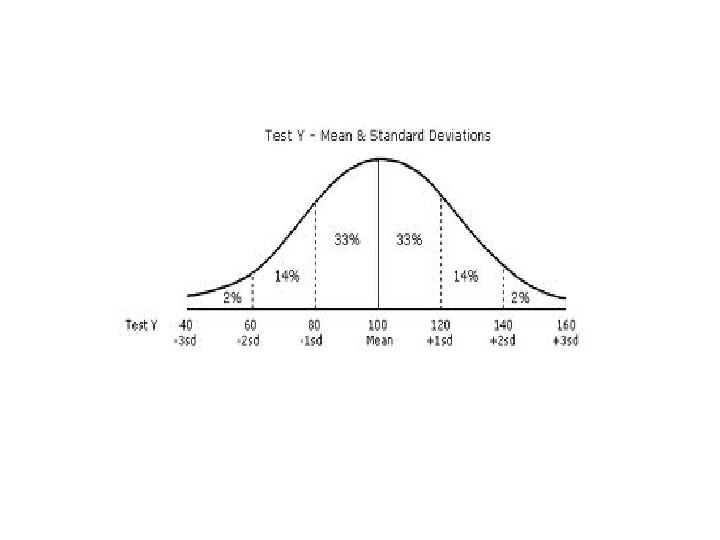
CONTINUOUS PROBABILITY • Mean : µ • Variance : σ2 same mean, different std dev • P(x 1 < µ < X 2) = P (z 1 < Z < z 2) z = (X-µ)/σ

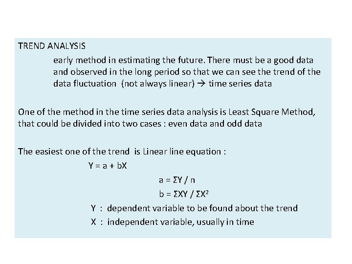
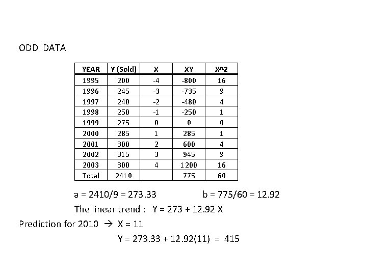
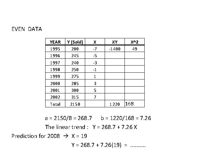
TREND ANALYSIS early method in estimating the future. There must be a good data and observed in the long period so that we can see the trend of the data fluctuation (not always linear) time series data One of the method in the time series data analysis is Least Square Method, that could be divided into two cases : even data and odd data The easiest one of the trend is Linear line equation : Y = a + b. X a = ΣY / n b = ΣXY / ΣX 2 Y : dependent variable to be found about the trend X : independent variable, usually in time

ODD DATA YEAR 1995 1996 1997 1998 1999 2000 2001 2002 2003 Total Y (Sold) 200 245 240 250 275 285 300 315 300 2410 X -4 -3 -2 -1 0 1 2 3 4 XY -800 -735 -480 -250 0 285 600 945 1200 775 X^2 16 9 4 1 0 1 4 9 16 60 a = 2410/9 = 273. 33 b = 775/60 = 12. 92 The linear trend : Y = 273 + 12. 92 X Prediction for 2010 X = 11 Y = 273. 33 + 12. 92(11) = 415

EVEN DATA YEAR 1995 1996 1997 1998 1999 2000 2001 2002 Total Y (Sold) 200 245 240 250 275 285 300 315 2150 X -7 -5 -3 -1 1 3 5 7 XY -1400 1220 X^2 49 168 a = 2150/8 = 268. 7 b = 1220/168 = 7. 26 The linear trend : Y = 268. 7 + 7. 26 X Prediction for 2008 X = 19 Y = 268. 7 + 7. 26(19) =. .

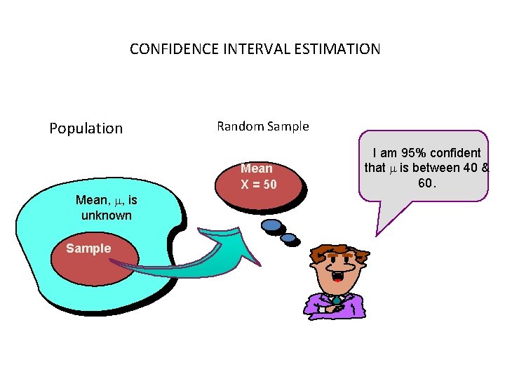
CONFIDENCE INTERVAL ESTIMATION Population Mean, , is unknown Sample Random Sample Mean X = 50 I am 95% confident that is between 40 & 60.

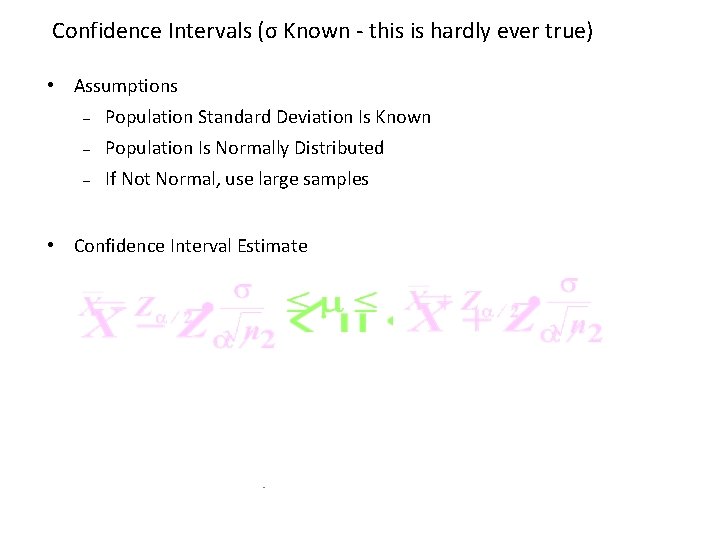
Confidence Intervals (σ Known - this is hardly ever true) • Assumptions – Population Standard Deviation Is Known – Population Is Normally Distributed – If Not Normal, use large samples • Confidence Interval Estimate

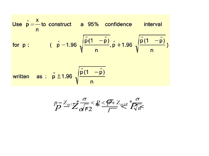
Shortcoming of Point Estimates ^ p= , the sample proportion of x successes in a sample of size n, is the best point estimate of the unknown value of the population proportion p E. g ^p = 590/1000 =. 59, best estimate of population proportion p BUT How good is this best estimate? A confidence interval is a range (or an interval) of values used to estimate the unknown value of a population parameter.

Tool for Constructing Confidence Intervals: The Central Limit Theorem • If a random sample of n observations is selected from a population (any population), and x “successes” are observed, then when n is sufficiently large, the sampling distribution of the sample proportion p will be approximately a normal distribution. • n is large when np ≥ 15 and nq ≥ 15.

HYPOTHESIS TESTING OF THE POPULATION MEAN

FUNDAMENTAL We use samples to learn about populations We seldom observe the populations we want to know about Because we have to use samples, we engage in inference from samples to populations However, because of sampling variability, samples are not little mirror images of the population of interest. Given that samples are imperfect replications of populations, we have to use techniques such as HYPOTHESIS TESTING to determine if statements about populations are reasonable given our observed population

INTRODUCTION Objective : to determine whether the parameter is significantly different with statistic Population mean = sample mean ?

DEFINITION Hypothesis H 0 : “no change” situation (hope to be disproved) H 1 : statement hoped to establish Statistical test procedure in making decision : accept H 0 or reject it (use for defining the hypothesis region) Types of error significance level α : 5% , 1% Direction of research hypothesis one-tailed test two-tailed test

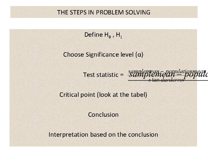
THE STEPS IN PROBLEM SOLVING Define H 0 , H 1 Choose Significance level (α) Test statistic = Critical point (look at the tabel) Conclusion Interpretation based on the conclusion

EXAMPLE : OBESITY

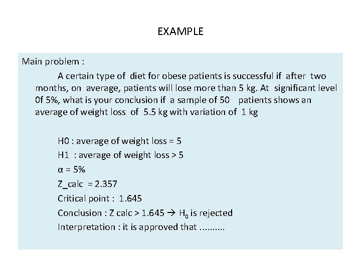
EXAMPLE Main problem : A certain type of diet for obese patients is successful if after two months, on average, patients will lose more than 5 kg. At significant level 0 f 5%, what is your conclusion if a sample of 50 patients shows an average of weight loss of 5. 5 kg with variation of 1 kg H 0 : average of weight loss = 5 H 1 : average of weight loss > 5 α = 5% Z_calc = 2. 357 Critical point : 1. 645 Conclusion : Z calc > 1. 645 H 0 is rejected Interpretation : it is approved that. .