General Game Playing Lecture 2 Game Description Michael

General Game Playing Lecture 2 Game Description Michael Genesereth Spring 2011

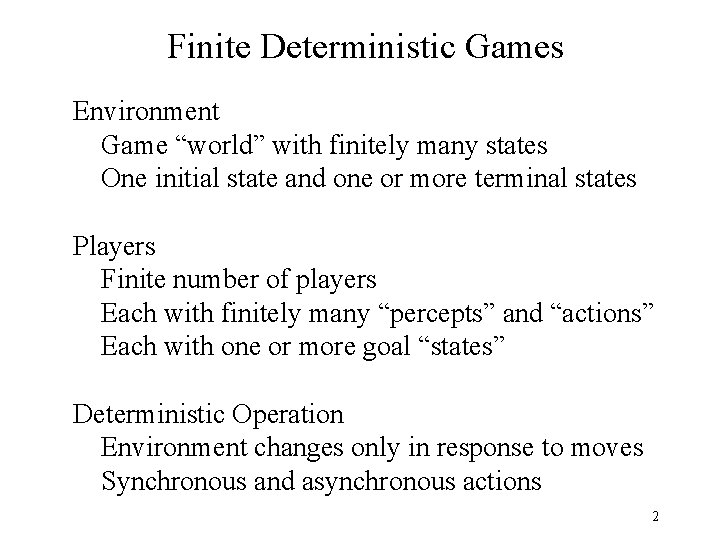
Finite Deterministic Games Environment Game “world” with finitely many states One initial state and one or more terminal states Players Finite number of players Each with finitely many “percepts” and “actions” Each with one or more goal “states” Deterministic Operation Environment changes only in response to moves Synchronous and asynchronous actions 2

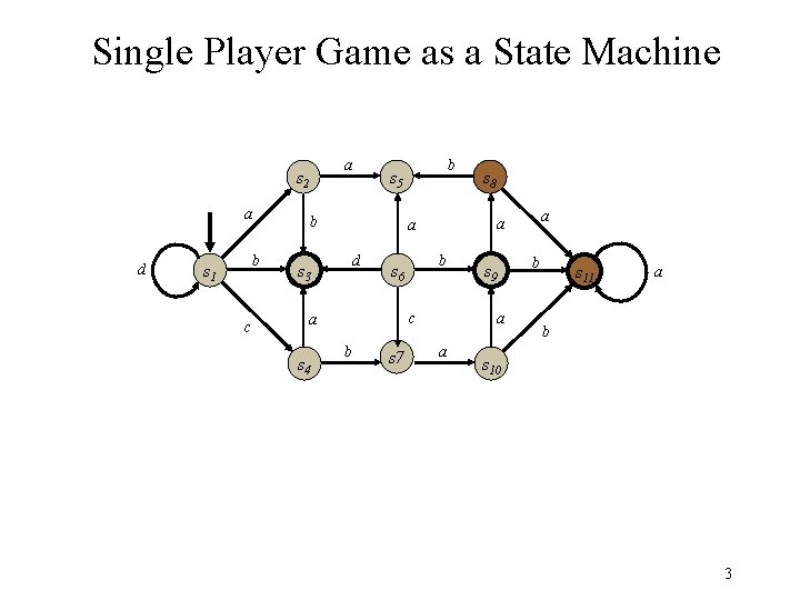
Single Player Game as a State Machine a s 2 a d b s 1 c b d b s 6 c a b s 7 s 8 a a a s 3 s 4 b s 5 s 9 a a b s 11 a b s 10 3

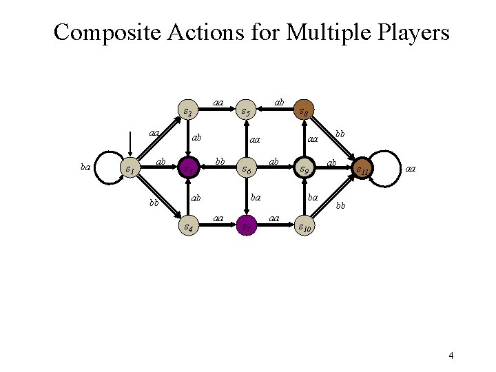
Composite Actions for Multiple Players aa s 2 aa ba s 1 ab bb ab s 3 ab s 5 ab s 6 ba ab s 4 aa aa bb aa s 7 s 8 s 9 ba aa bb ab s 11 aa bb s 10 4

Problem Since all of the games that we are considering are finite, it is possible in principle to communicate game information in the form of transition graphs. Problem: Size of description. Even though everything is finite, the graphs can be large. 5

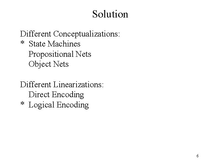
Solution Different Conceptualizations: * State Machines Propositional Nets Object Nets Different Linearizations: Direct Encoding * Logical Encoding 6

Game Description Language 7

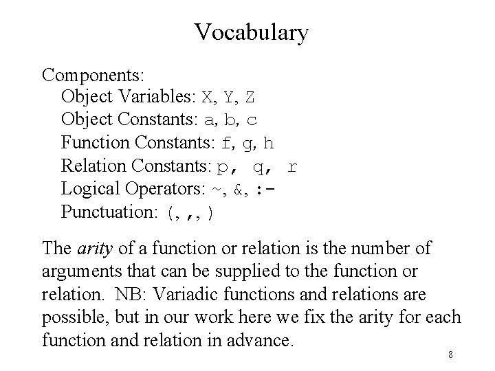
Vocabulary Components: Object Variables: X, Y, Z Object Constants: a, b, c Function Constants: f, g, h Relation Constants: p, q, r Logical Operators: ~, &, : Punctuation: (, , , ) The arity of a function or relation is the number of arguments that can be supplied to the function or relation. NB: Variadic functions and relations are possible, but in our work here we fix the arity for each function and relation in advance. 8

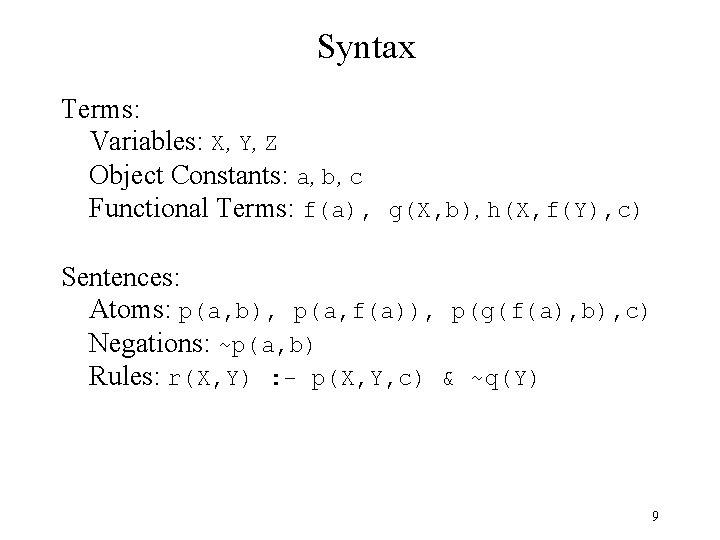
Syntax Terms: Variables: X, Y, Z Object Constants: a, b, c Functional Terms: f(a), g(X, b), h(X, f(Y), c) Sentences: Atoms: p(a, b), p(a, f(a)), p(g(f(a), b), c) Negations: ~p(a, b) Rules: r(X, Y) : - p(X, Y, c) & ~q(Y) 9

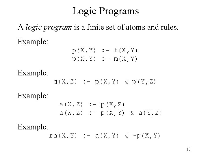
Logic Programs A logic program is a finite set of atoms and rules. Example: p(X, Y) : - f(X, Y) p(X, Y) : - m(X, Y) Example: g(X, Z) : - p(X, Y) & p(Y, Z) Example: a(X, Z) : - p(X, Z) a(X, Z) : - p(X, Y) & a(Y, Z) Example: ra(X, Y) : - a(X, Y) & ~p(X, Y) 10

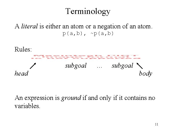
Terminology A literal is either an atom or a negation of an atom. p(a, b), ~p(a, b) Rules: subgoal head … subgoal body An expression is ground if and only if it contains no variables. 11

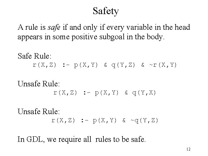
Safety A rule is safe if and only if every variable in the head appears in some positive subgoal in the body. Safe Rule: r(X, Z) : - p(X, Y) & q(Y, Z) & ~r(X, Y) Unsafe Rule: r(X, Z) : - p(X, Y) & q(Y, X) Unsafe Rule: r(X, Z) : - p(X, Y) & ~q(Y, Z) In GDL, we require all rules to be safe. 12

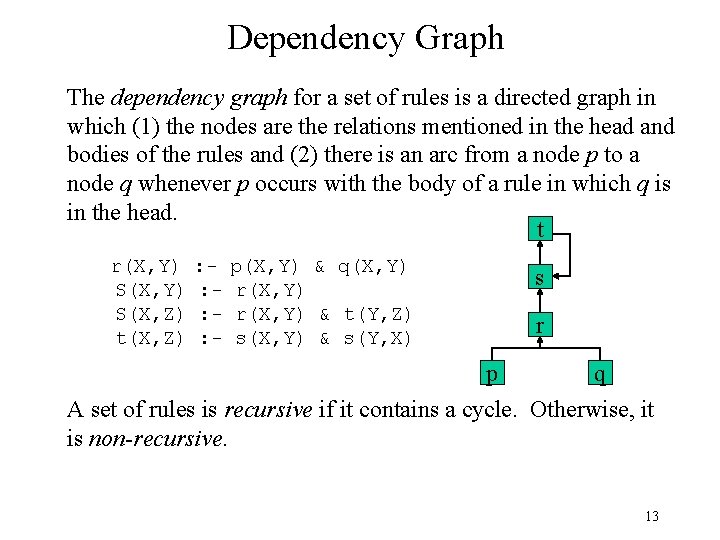
Dependency Graph The dependency graph for a set of rules is a directed graph in which (1) the nodes are the relations mentioned in the head and bodies of the rules and (2) there is an arc from a node p to a node q whenever p occurs with the body of a rule in which q is in the head. t r(X, Y) S(X, Z) t(X, Z) : : - p(X, Y) & q(X, Y) r(X, Y) & t(Y, Z) s(X, Y) & s(Y, X) s r p q A set of rules is recursive if it contains a cycle. Otherwise, it is non-recursive. 13

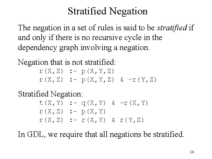
Stratified Negation The negation in a set of rules is said to be stratified if and only if there is no recursive cycle in the dependency graph involving a negation. Negation that is not stratified: r(X, Z) : - p(X, Y, Z) & ~r(Y, Z) Stratified Negation: t(X, Y) : - q(X, Y) & ~r(X, Y) r(X, Z) : - p(X, Y) r(X, Z) : - r(X, Y) & r(Y, Z) In GDL, we require that all negations be stratified. 14

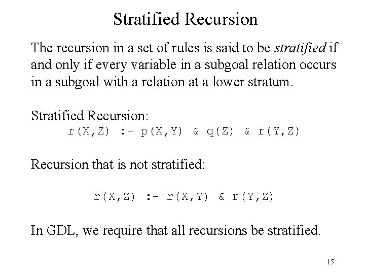
Stratified Recursion The recursion in a set of rules is said to be stratified if and only if every variable in a subgoal relation occurs in a subgoal with a relation at a lower stratum. Stratified Recursion: r(X, Z) : - p(X, Y) & q(Z) & r(Y, Z) Recursion that is not stratified: r(X, Z) : - r(X, Y) & r(Y, Z) In GDL, we require that all recursions be stratified. 15

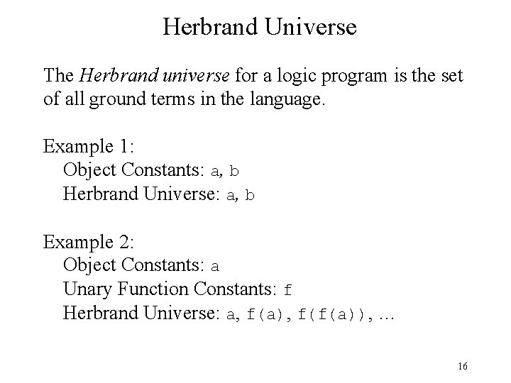
Herbrand Universe The Herbrand universe for a logic program is the set of all ground terms in the language. Example 1: Object Constants: a, b Herbrand Universe: a, b Example 2: Object Constants: a Unary Function Constants: f Herbrand Universe: a, f(a), f(f(a)), … 16

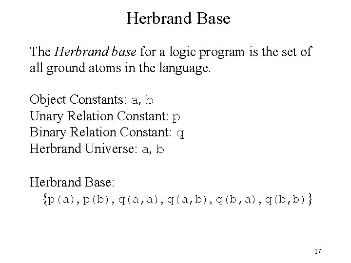
Herbrand Base The Herbrand base for a logic program is the set of all ground atoms in the language. Object Constants: a, b Unary Relation Constant: p Binary Relation Constant: q Herbrand Universe: a, b Herbrand Base: {p(a), p(b), q(a, a), q(a, b), q(b, a), q(b, b)} 17

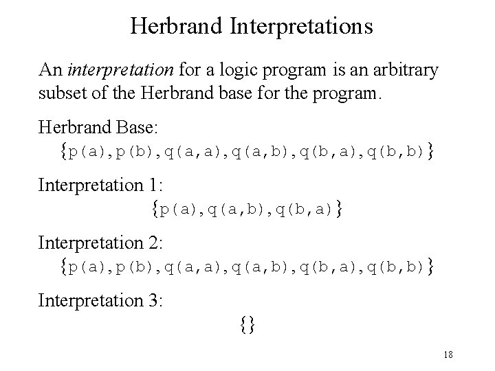
Herbrand Interpretations An interpretation for a logic program is an arbitrary subset of the Herbrand base for the program. Herbrand Base: {p(a), p(b), q(a, a), q(a, b), q(b, a), q(b, b)} Interpretation 1: {p(a), q(a, b), q(b, a)} Interpretation 2: {p(a), p(b), q(a, a), q(a, b), q(b, a), q(b, b)} Interpretation 3: {} 18

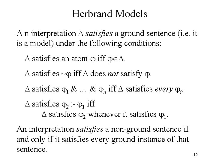
Herbrand Models A n interpretation satisfies a ground sentence (i. e. it is a model) under the following conditions: satisfies an atom iff . satisfies ~ iff does not satisfy . satisfies 1 & … & n iff satisfies every i. satisfies 2 : - 1 iff satisfies 2 whenever it satisfies 1. An interpretation satisfies a non-ground sentence if and only if it satisfies every ground instance of that sentence. 19

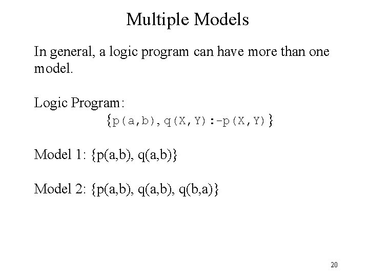
Multiple Models In general, a logic program can have more than one model. Logic Program: {p(a, b), q(X, Y): -p(X, Y)} Model 1: {p(a, b), q(a, b)} Model 2: {p(a, b), q(b, a)} 20

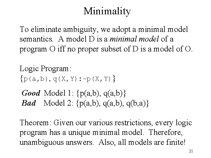
Minimality To eliminate ambiguity, we adopt a minimal model semantics. A model D is a minimal model of a program O iff no proper subset of D is a model of O. Logic Program: {p(a, b), q(X, Y): -p(X, Y)} Good Model 1: {p(a, b), q(a, b)} Bad Model 2: {p(a, b), q(b, a)} Theorem: Given our various restrictions, every logic program has a unique minimal model. Therefore, unambiguous answers. Also, all models are finite! 21

Open versus Closed Logic Programs Logic programs as just defined are closed in that they fix the meaning of all relations. In open logic programs, some of the relations are given as inputs (rather than being defined) and other relations are produced as outputs (defined in terms of the inputs). In other words, open logic programs can be used with different input datasets to produce different output datasets. 22

Open Logic Programs An open logic program is a logic program together with a partition of the relations into two types - base relations (the inputs) and view relations (the defined relations). View relations can appear anywhere in the program, while base relations can appear only in the bodies of rules (never in the heads of rules). 23

Inputs and Outputs An overall model of an open logic program O with an input model D is is the minimal model of O D. The output of an open logic program for input D is the subset of the overall model of O and D that mentions only output relations. 24

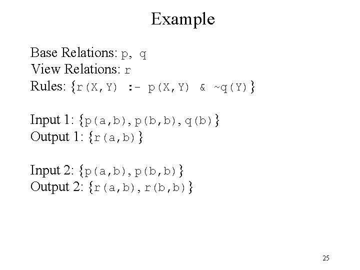
Example Base Relations: p, q View Relations: r Rules: {r(X, Y) : - p(X, Y) & ~q(Y)} Input 1: {p(a, b), p(b, b), q(b)} Output 1: {r(a, b)} Input 2: {p(a, b), p(b, b)} Output 2: {r(a, b), r(b, b)} 25

26

GDL 27

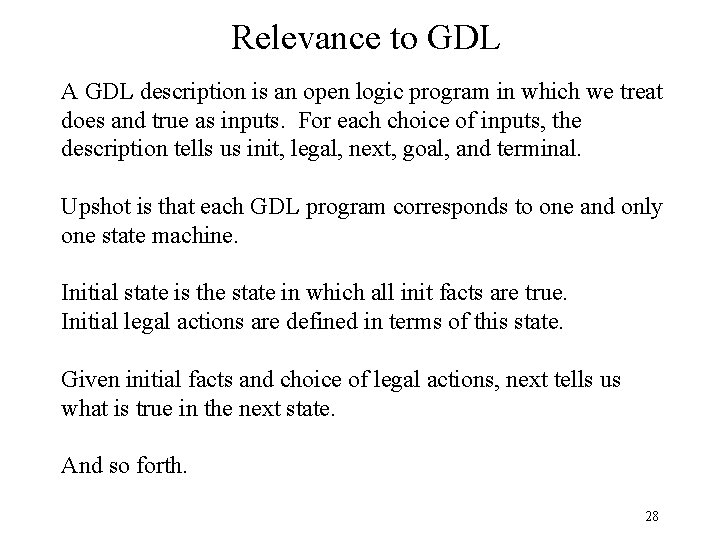
Relevance to GDL A GDL description is an open logic program in which we treat does and true as inputs. For each choice of inputs, the description tells us init, legal, next, goal, and terminal. Upshot is that each GDL program corresponds to one and only one state machine. Initial state is the state in which all init facts are true. Initial legal actions are defined in terms of this state. Given initial facts and choice of legal actions, next tells us what is true in the next state. And so forth. 28

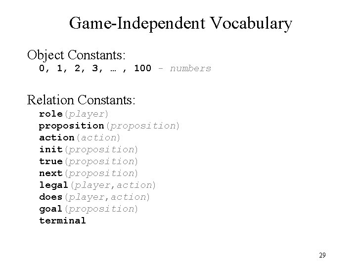
Game-Independent Vocabulary Object Constants: 0, 1, 2, 3, … , 100 - numbers Relation Constants: role(player) proposition(proposition) action(action) init(proposition) true(proposition) next(proposition) legal(player, action) does(player, action) goal(proposition) terminal 29

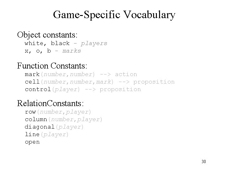
Game-Specific Vocabulary Object constants: white, black - players x, o, b - marks Function Constants: mark(number, number) --> action cell(number, mark) --> proposition control(player) --> proposition Relation. Constants: row(number, player) column(number, player) diagonal(player) line(player) open 30

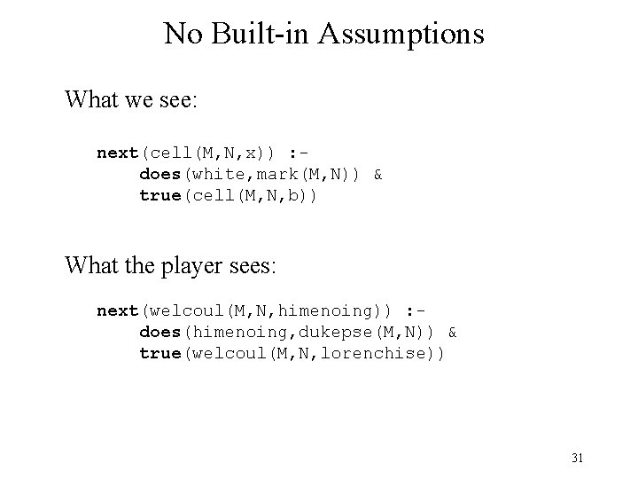
No Built-in Assumptions What we see: next(cell(M, N, x)) : does(white, mark(M, N)) & true(cell(M, N, b)) What the player sees: next(welcoul(M, N, himenoing)) : does(himenoing, dukepse(M, N)) & true(welcoul(M, N, lorenchise)) 31

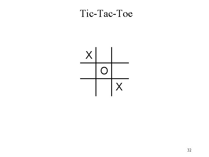
Tic-Tac-Toe X O X 32

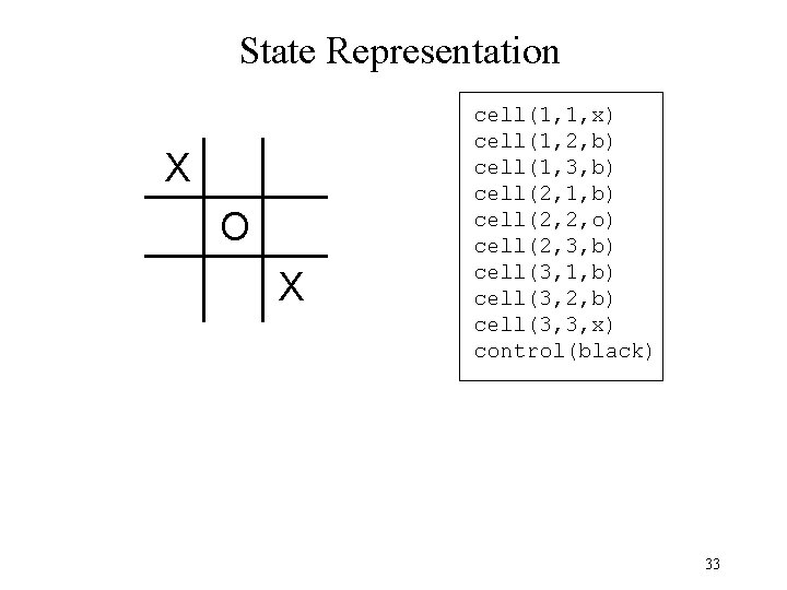
State Representation X O X cell(1, 1, x) cell(1, 2, b) cell(1, 3, b) cell(2, 1, b) cell(2, 2, o) cell(2, 3, b) cell(3, 1, b) cell(3, 2, b) cell(3, 3, x) control(black) 33

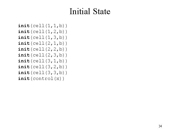
Initial State init(cell(1, 1, b)) init(cell(1, 2, b)) init(cell(1, 3, b)) init(cell(2, 1, b)) init(cell(2, 2, b)) init(cell(2, 3, b)) init(cell(3, 1, b)) init(cell(3, 2, b)) init(cell(3, 3, b)) init(control(x)) 34

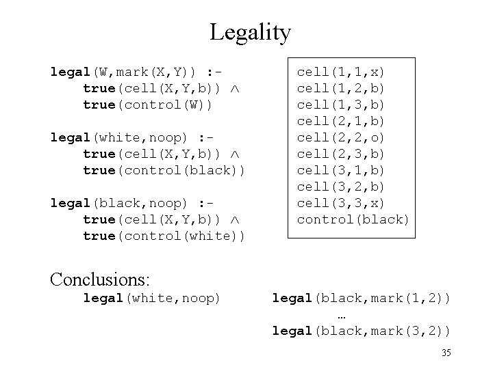
Legality legal(W, mark(X, Y)) : true(cell(X, Y, b)) true(control(W)) legal(white, noop) : true(cell(X, Y, b)) true(control(black)) legal(black, noop) : true(cell(X, Y, b)) true(control(white)) cell(1, 1, x) cell(1, 2, b) cell(1, 3, b) cell(2, 1, b) cell(2, 2, o) cell(2, 3, b) cell(3, 1, b) cell(3, 2, b) cell(3, 3, x) control(black) Conclusions: legal(white, noop) legal(black, mark(1, 2)) … legal(black, mark(3, 2)) 35

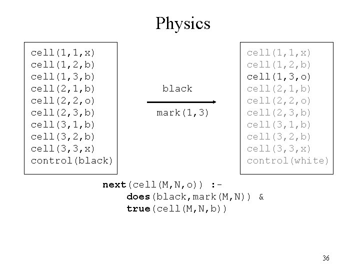
Physics cell(1, 1, x) cell(1, 2, b) cell(1, 3, b) cell(2, 1, b) cell(2, 2, o) cell(2, 3, b) cell(3, 1, b) cell(3, 2, b) cell(3, 3, x) control(black) black mark(1, 3) cell(1, 1, x) cell(1, 2, b) cell(1, 3, o) cell(2, 1, b) cell(2, 2, o) cell(2, 3, b) cell(3, 1, b) cell(3, 2, b) cell(3, 3, x) control(white) next(cell(M, N, o)) : does(black, mark(M, N)) & true(cell(M, N, b)) 36

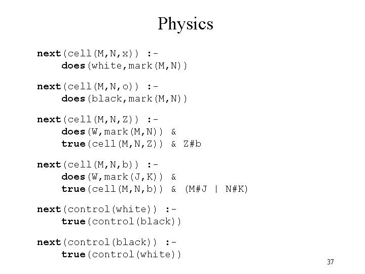
Physics next(cell(M, N, x)) : does(white, mark(M, N)) next(cell(M, N, o)) : does(black, mark(M, N)) next(cell(M, N, Z)) : does(W, mark(M, N)) & true(cell(M, N, Z)) & Z#b next(cell(M, N, b)) : does(W, mark(J, K)) & true(cell(M, N, b)) & (M#J | N#K) next(control(white)) : true(control(black)) next(control(black)) : true(control(white)) 37

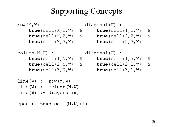
Supporting Concepts row(M, W) : diagonal(W) : true(cell(M, 1, W)) & true(cell(1, 1, W)) & true(cell(M, 2, W)) & true(cell(2, 2, W)) & true(cell(M, 3, W)) true(cell(3, 3, W)) column(N, W) : diagonal(W) : true(cell(1, N, W)) & true(cell(1, 3, W)) & true(cell(2, N, W)) & true(cell(2, 2, W)) & true(cell(3, N, W)) true(cell(3, 1, W)) line(W) : - row(M, W) line(W) : - column(N, W) line(W) : - diagonal(W) open : - true(cell(M, N, b)) 38

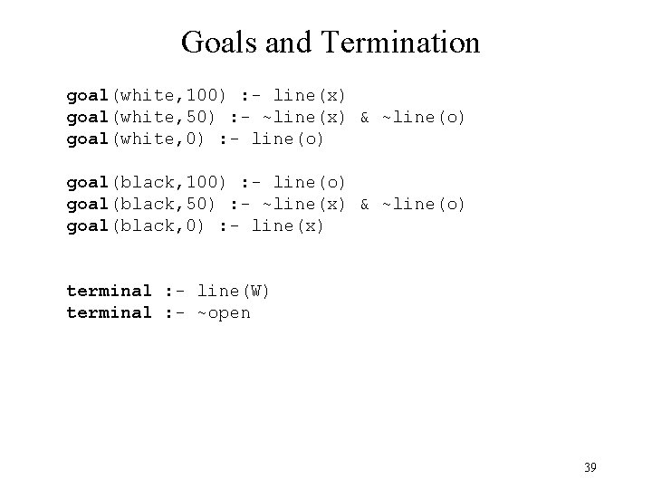
Goals and Termination goal(white, 100) : - line(x) goal(white, 50) : - ~line(x) & ~line(o) goal(white, 0) : - line(o) goal(black, 100) : - line(o) goal(black, 50) : - ~line(x) & ~line(o) goal(black, 0) : - line(x) terminal : - line(W) terminal : - ~open 39

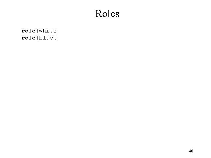
Roles role(white) role(black) 40

GGP Details 41

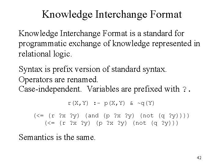
Knowledge Interchange Format is a standard for programmatic exchange of knowledge represented in relational logic. Syntax is prefix version of standard syntax. Operators are renamed. Case-independent. Variables are prefixed with ? . r(X, Y) : - p(X, Y) & ~q(Y) (<= (r ? x ? y) (and (p ? x ? y) (not (q ? y)))) (<= (r ? x ? y) (p ? x ? y) (not (q ? y))) Semantics is the same. 42

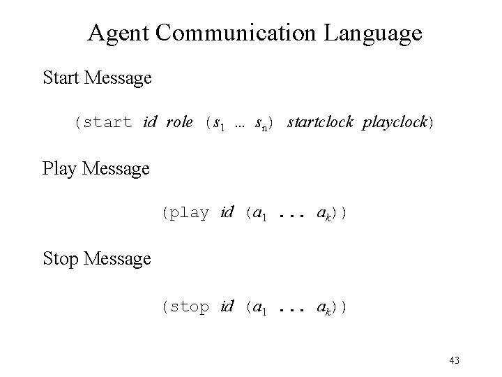
Agent Communication Language Start Message (start id role (s 1 … sn) startclock playclock) Play Message (play id (a 1. . . ak)) Stop Message (stop id (a 1. . . ak)) 43

Completeness Of necessity, game descriptions are logically incomplete in that they do not uniquely specify the moves of the players. Every game description contains complete definitions for legality, termination, goalhood, and update in terms of the primitive moves and the does relation. The upshot is that in every state every player can determine legality, termination, goalhood and, given a joint move, can update the state. 44

Playability A game is playable if and only if every player has at least one legal move in every non-terminal state. Note that in chess, if a player cannot move, it is a stalemate. Fortunately, this is a terminal state. In GGP, we guarantee that every game is playable. 45

Winnability A game is strongly winnable if and only if, for some player, there is a sequence of individual moves of that player that leads to a terminating goal state for that player. A game is weakly winnable if and only if, for every player, there is a sequence of joint moves of the players that leads to a terminating goal state for that player. In GGP, every game is weakly winnable, and all single player games are strongly winnable. 46

47

48