FORECASTING Qualitative Analysis Quantitative Analysis Predictions or Forecasting

FORECASTING Qualitative Analysis ~ Quantitative Analysis

Predictions or Forecasting with: -Multiple Regression -Confidence Interval for Prediction -Trend Analysis and Projections -Seasonal Models -Smoothing Techniques

Qualitative Analysis -Surveys -Polling -Expert Opinion (Personal Insight) -Panel Consensus -Delphi method • using forecasts derived from independent analysis of expert opinion

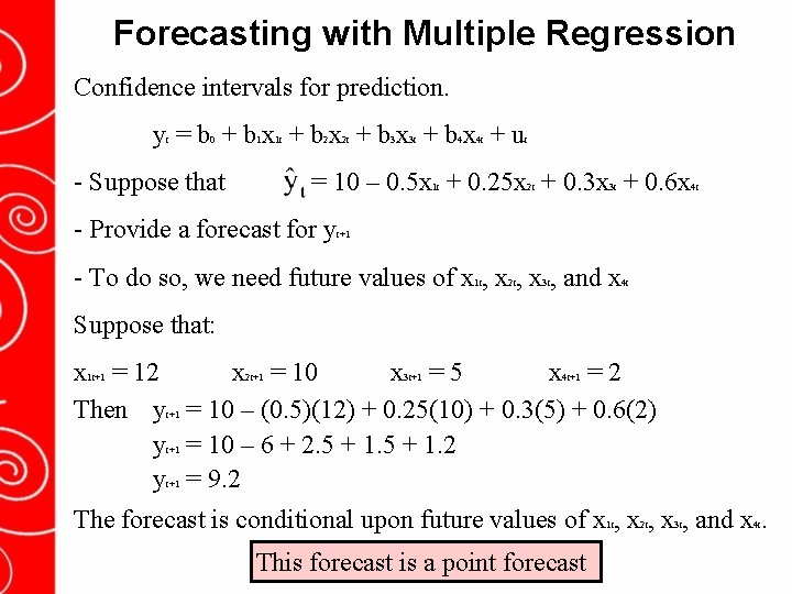
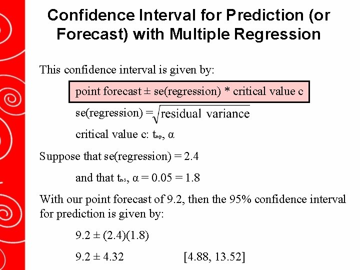
Forecasting with Multiple Regression Confidence intervals for prediction. y = b + bx + u t 0 1 - Suppose that 1 t 2 2 t 3 3 t 4 4 t t = 10 – 0. 5 x + 0. 25 x + 0. 3 x + 0. 6 x 1 t - Provide a forecast for y 2 t 3 t 4 t t+1 - To do so, we need future values of x , x , and x 1 t 2 t 3 t 4 t Suppose that: x = 12 x = 10 x =5 x =2 Then y = 10 – (0. 5)(12) + 0. 25(10) + 0. 3(5) + 0. 6(2) y = 10 – 6 + 2. 5 + 1. 2 y = 9. 2 1 t+1 2 t+1 3 t+1 4 t+1 t+1 The forecast is conditional upon future values of x , x , and x. 1 t This forecast is a point forecast 2 t 3 t 4 t

Confidence Interval for Prediction (or Forecast) with Multiple Regression This confidence interval is given by: point forecast ± se(regression) * critical value c se(regression) = critical value c: t , α n-p Suppose that se(regression) = 2. 4 and that t , α = 0. 05 = 1. 8 n-5 With our point forecast of 9. 2, then the 95% confidence interval for prediction is given by: 9. 2 ± (2. 4)(1. 8) 9. 2 ± 4. 32 [4. 88, 13. 52]

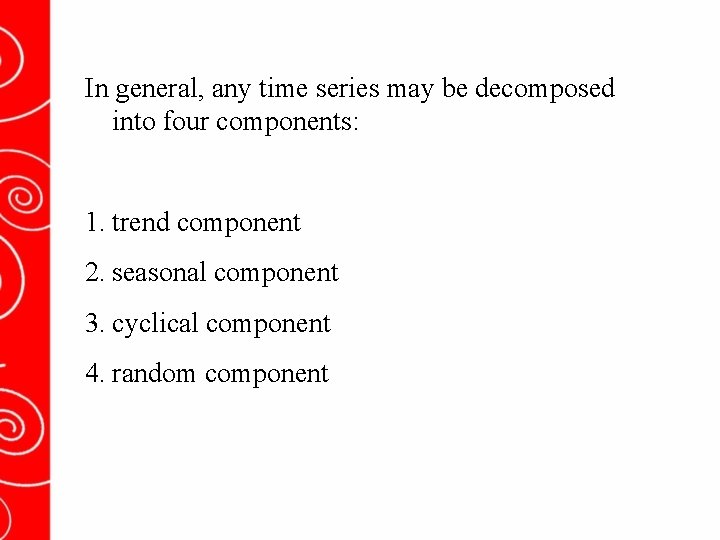
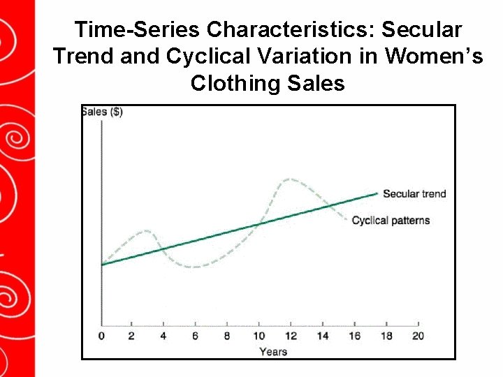
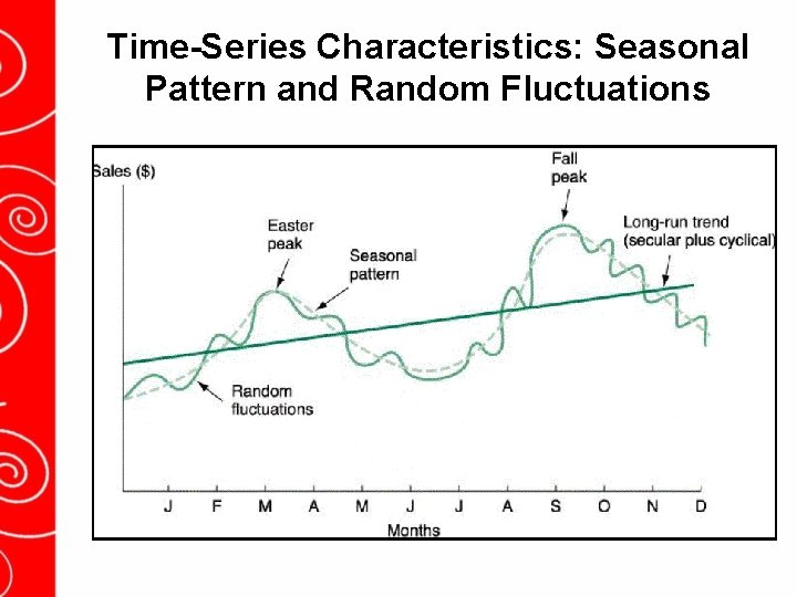
In general, any time series may be decomposed into four components: 1. trend component 2. seasonal component 3. cyclical component 4. random component

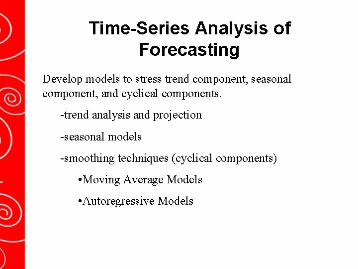
Time-Series Analysis of Forecasting Develop models to stress trend component, seasonal component, and cyclical components. -trend analysis and projection -seasonal models -smoothing techniques (cyclical components) • Moving Average Models • Autoregressive Models

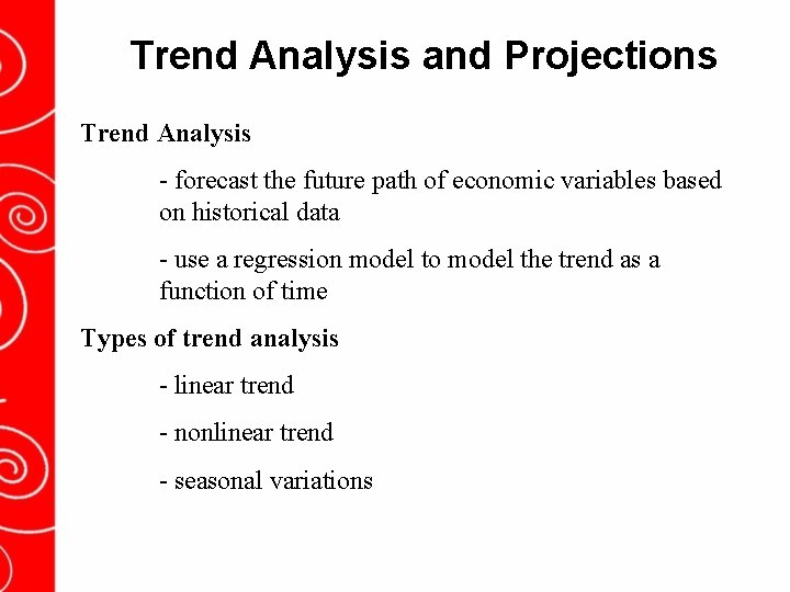
Trend Analysis and Projections Trend Analysis - forecast the future path of economic variables based on historical data - use a regression model to model the trend as a function of time Types of trend analysis - linear trend - nonlinear trend - seasonal variations

Time-Series Characteristics: Secular Trend and Cyclical Variation in Women’s Clothing Sales

Time-Series Characteristics: Seasonal Pattern and Random Fluctuations

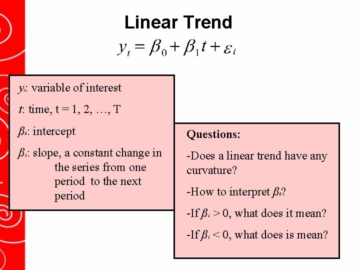
Linear Trend y : variable of interest t t: time, t = 1, 2, …, T ß : intercept Questions: ß : slope, a constant change in the series from one period to the next period -Does a linear trend have any curvature? 0 1 -How to interpret ß ? 0 -If ß > 0, what does it mean? 1 -If ß < 0, what does is mean? 1

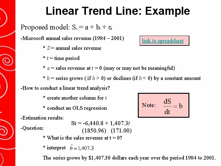
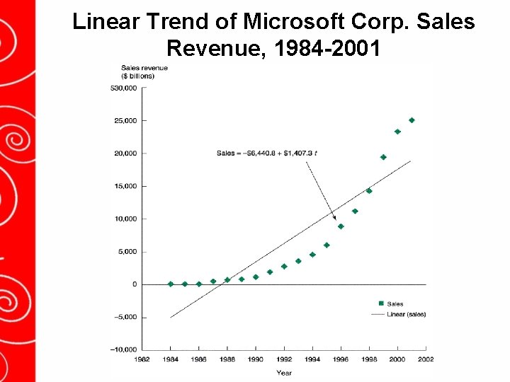
Linear Trend Line: Example Proposed model: S = a + b + ε t t t -Microsoft annual sales revenue (1984 – 2001) link to spreadsheet * S = annual sales revenue * t = time period * a = sales revenue at t = 0 (may or may not be meaningful) * b = series grows ( if b > 0) or declines (if b < 0) by a constant amount -How to conduct a linear trend analysis? * create another column for t * conduct an OLS regression -Estimation results: -Question: Note: St = -6, 440. 8 + 1, 407. 3 t (1850. 96) (171. 00) * What is the sales revenue at t = 0? * interpret The series grows by $1, 407. 30 dollars each year over the period 1984 to 2001.

Linear Trend of Microsoft Corp. Sales Revenue, 1984 -2001

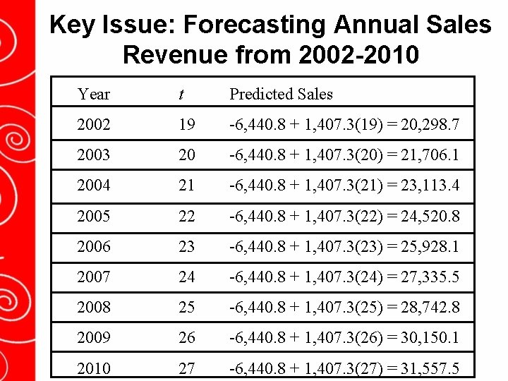
Key Issue: Forecasting Annual Sales Revenue from 2002 -2010 Year t Predicted Sales 2002 19 -6, 440. 8 + 1, 407. 3(19) = 20, 298. 7 2003 20 -6, 440. 8 + 1, 407. 3(20) = 21, 706. 1 2004 21 -6, 440. 8 + 1, 407. 3(21) = 23, 113. 4 2005 22 -6, 440. 8 + 1, 407. 3(22) = 24, 520. 8 2006 23 -6, 440. 8 + 1, 407. 3(23) = 25, 928. 1 2007 24 -6, 440. 8 + 1, 407. 3(24) = 27, 335. 5 2008 25 -6, 440. 8 + 1, 407. 3(25) = 28, 742. 8 2009 26 -6, 440. 8 + 1, 407. 3(26) = 30, 150. 1 2010 27 -6, 440. 8 + 1, 407. 3(27) = 31, 557. 5

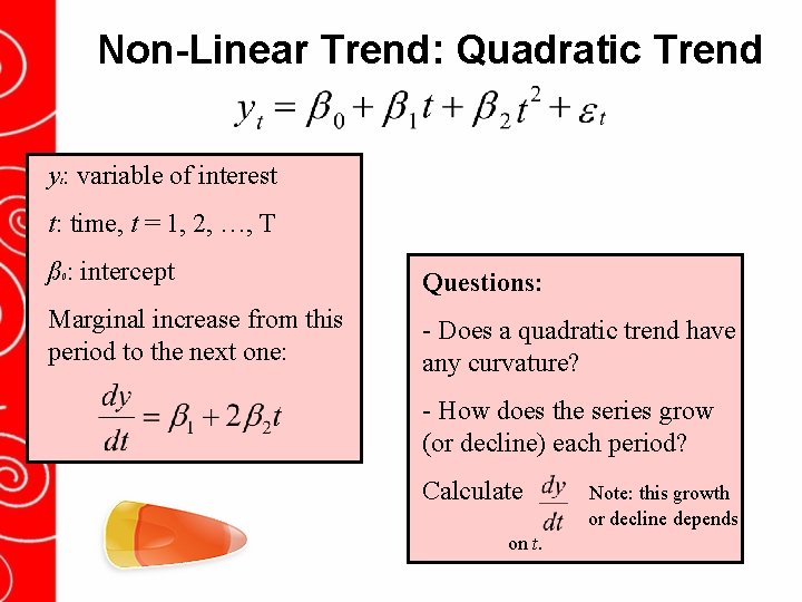
Non-Linear Trend: Quadratic Trend y : variable of interest t t: time, t = 1, 2, …, T ß : intercept Questions: Marginal increase from this period to the next one: - Does a quadratic trend have any curvature? 0 - How does the series grow (or decline) each period? Calculate on t. Note: this growth or decline depends

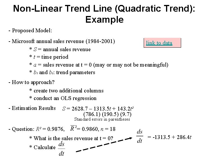
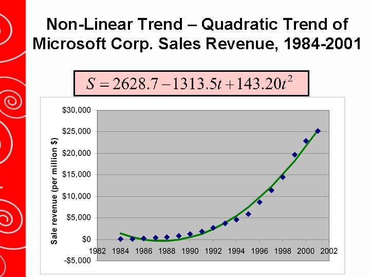
Non-Linear Trend Line (Quadratic Trend): Example - Proposed Model: - Microsoft annual sales revenue (1984 -2001) link to data * S = annual sales revenue * t = time period * a = sales revenue at t = 0 (may or may not be meaningful) * b and b : trend parameters 1 2 - How to approach? * create two additional columns * conduct an OLS regression - Estimation Results S = 2628. 7 – 1313. 5 t + 143. 2 t² (786. 1) (190. 5) (9. 7) Standard errors in parentheses - Question: R² = 0. 9876, = 0. 9860, n = 18 * What is the sales revenue at t = 0? * Calculate = -1313. 5 + 286. 4 t

Non-Linear Trend – Quadratic Trend of Microsoft Corp. Sales Revenue, 1984 -2001

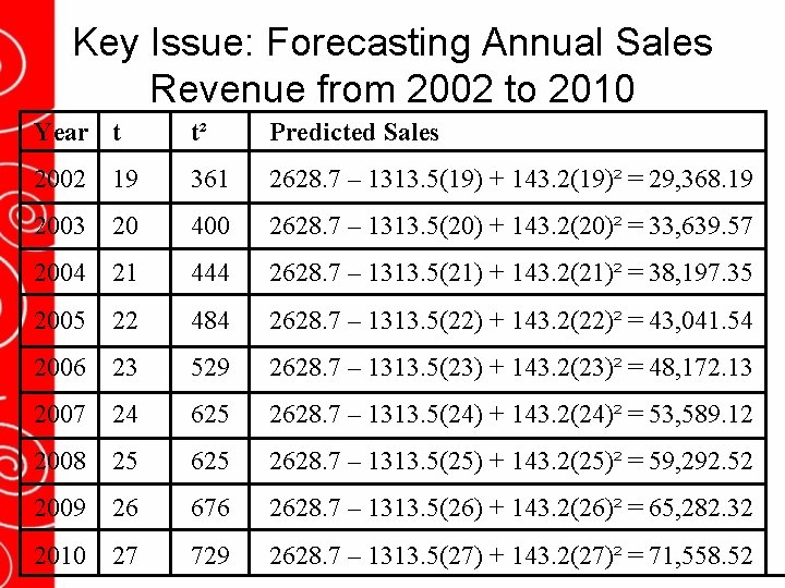
Key Issue: Forecasting Annual Sales Revenue from 2002 to 2010 Year t t² Predicted Sales 2002 19 361 2628. 7 – 1313. 5(19) + 143. 2(19)² = 29, 368. 19 2003 20 400 2628. 7 – 1313. 5(20) + 143. 2(20)² = 33, 639. 57 2004 21 444 2628. 7 – 1313. 5(21) + 143. 2(21)² = 38, 197. 35 2005 22 484 2628. 7 – 1313. 5(22) + 143. 2(22)² = 43, 041. 54 2006 23 529 2628. 7 – 1313. 5(23) + 143. 2(23)² = 48, 172. 13 2007 24 625 2628. 7 – 1313. 5(24) + 143. 2(24)² = 53, 589. 12 2008 25 625 2628. 7 – 1313. 5(25) + 143. 2(25)² = 59, 292. 52 2009 26 676 2628. 7 – 1313. 5(26) + 143. 2(26)² = 65, 282. 32 2010 27 729 2628. 7 – 1313. 5(27) + 143. 2(27)² = 71, 558. 52

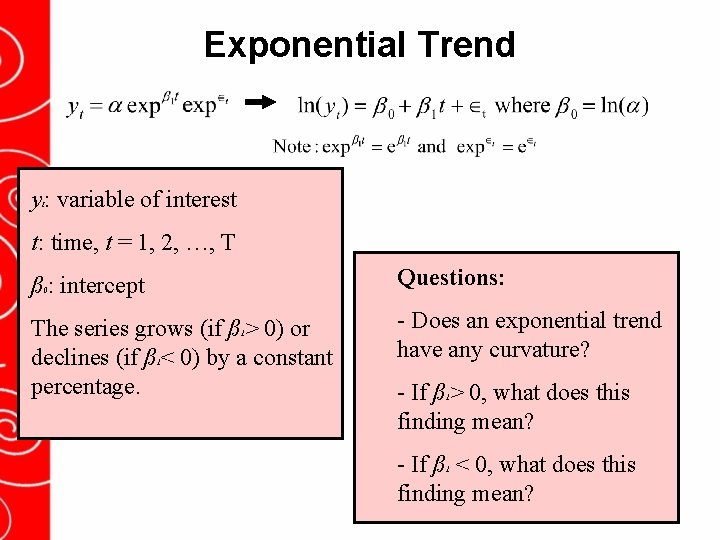
Exponential Trend y : variable of interest t t: time, t = 1, 2, …, T Questions: ß : intercept 0 The series grows (if ß > 0) or declines (if ß < 0) by a constant percentage. 1 1 - Does an exponential trend have any curvature? - If ß > 0, what does this finding mean? 1 - If ß < 0, what does this finding mean? 1

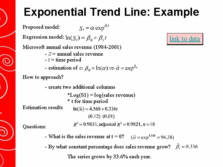
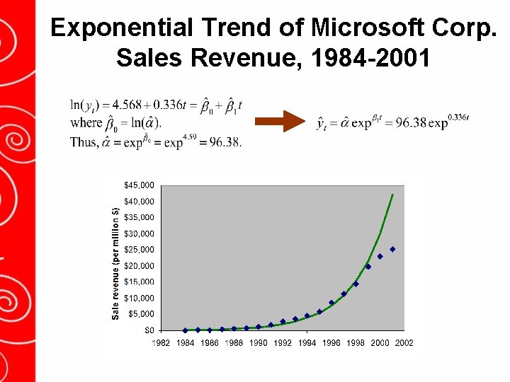
Exponential Trend Line: Example Proposed model: Regression model: link to data Microsoft annual sales revenue (1984 -2001) - S = annual sales revenue - t = time period - estimation of α: How to approach? - create two additional columns *Log(S 1) = log(sales revenue) * t for time period Estimation results Questions: - What is the sales revenue at t = 0? - By what constant percentage does sales revenue grow? The series grows by 33. 6% each year.

Exponential Trend of Microsoft Corp. Sales Revenue, 1984 -2001

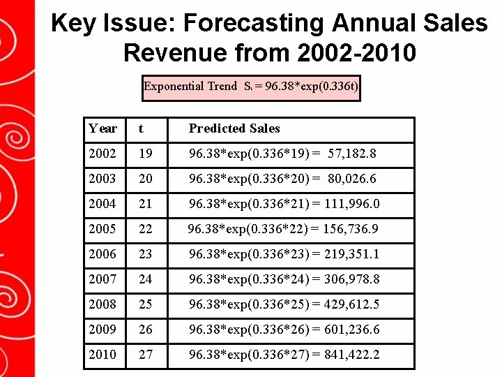
Key Issue: Forecasting Annual Sales Revenue from 2002 -2010 Exponential Trend S = 96. 38*exp(0. 336 t) t Year t Predicted Sales 2002 19 96. 38*exp(0. 336*19) = 57, 182. 8 2003 20 96. 38*exp(0. 336*20) = 80, 026. 6 2004 21 96. 38*exp(0. 336*21) = 111, 996. 0 2005 22 96. 38*exp(0. 336*22) = 156, 736. 9 2006 23 96. 38*exp(0. 336*23) = 219, 351. 1 2007 24 96. 38*exp(0. 336*24) = 306, 978. 8 2008 25 96. 38*exp(0. 336*25) = 429, 612. 5 2009 26 96. 38*exp(0. 336*26) = 601, 236. 6 2010 27 96. 38*exp(0. 336*27) = 841, 422. 2

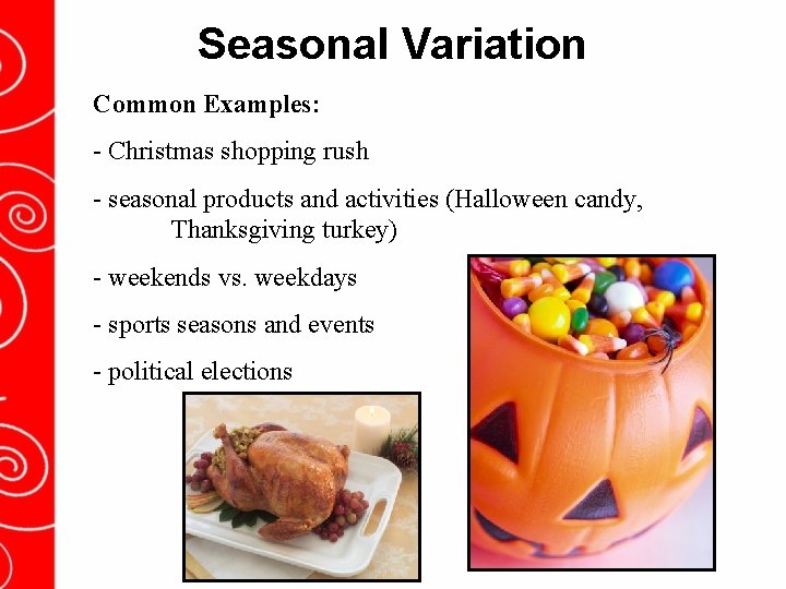
Seasonal Variation Common Examples: - Christmas shopping rush - seasonal products and activities (Halloween candy, Thanksgiving turkey) - weekends vs. weekdays - sports seasons and events - political elections

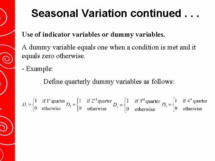
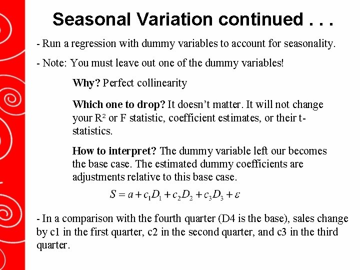
Seasonal Variation continued. . . Use of indicator variables or dummy variables. A dummy variable equals one when a condition is met and it equals zero otherwise. - Example: Define quarterly dummy variables as follows:

Seasonal Variation continued. . . - Run a regression with dummy variables to account for seasonality. - Note: You must leave out one of the dummy variables! Why? Perfect collinearity Which one to drop? It doesn’t matter. It will not change your R² or F statistic, coefficient estimates, or their tstatistics. How to interpret? The dummy variable left our becomes the base case. The estimated dummy coefficients are adjustments relative to this base case. - In a comparison with the fourth quarter (D 4 is the base), sales change by c 1 in the first quarter, c 2 in the second quarter, and c 3 in the third quarter.

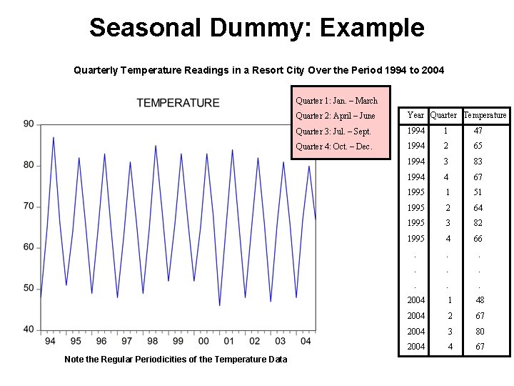
Seasonal Dummy: Example Quarterly Temperature Readings in a Resort City Over the Period 1994 to 2004 Quarter 1: Jan. – March Note the Regular Periodicities of the Temperature Data Quarter 2: April – June Year Quarter Temperature Quarter 3: Jul. – Sept. 1994 1 47 Quarter 4: Oct. – Dec. 1994 2 65 1994 3 83 1994 4 67 1995 1 51 1995 2 64 1995 3 82 1995 4 66 . . 2004 1 48 2004 2 67 2004 3 80 2004 4 67

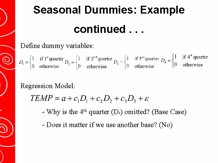
Seasonal Dummies: Example continued. . . Define dummy variables: Regression Model: - Why is the 4 th quarter (D ) omitted? (Base Case) 4 - Does it matter if we use another base? (No)

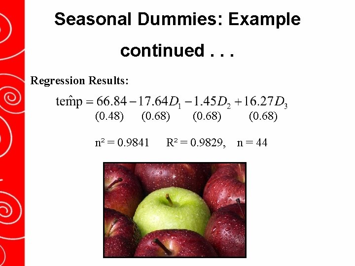
Seasonal Dummies: Example continued. . . Regression Results: (0. 48) (0. 68) n² = 0. 9841 (0. 68) R² = 0. 9829, n = 44

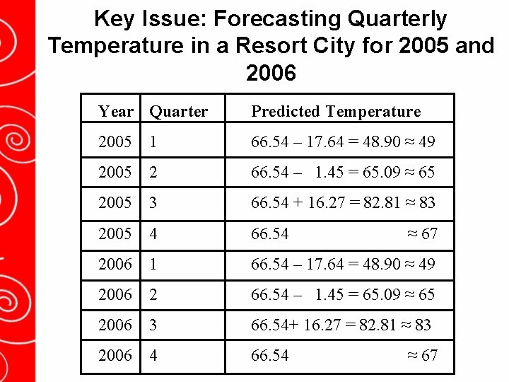
Key Issue: Forecasting Quarterly Temperature in a Resort City for 2005 and 2006 Year Quarter Predicted Temperature 2005 1 66. 54 – 17. 64 = 48. 90 ≈ 49 2005 2 66. 54 – 1. 45 = 65. 09 ≈ 65 2005 3 66. 54 + 16. 27 = 82. 81 ≈ 83 2005 4 66. 54 2006 1 66. 54 – 17. 64 = 48. 90 ≈ 49 2006 2 66. 54 – 1. 45 = 65. 09 ≈ 65 2006 3 66. 54+ 16. 27 = 82. 81 ≈ 83 2006 4 66. 54 ≈ 67

Smoothing Techniques - Take into account cyclical components in a time-series. - Smoothing Techniques: Moving Average model Autoregressive model

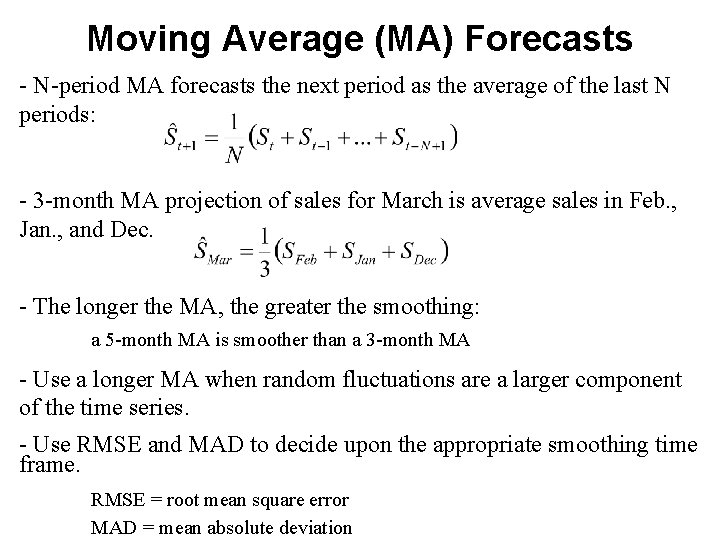
Moving Average (MA) Forecasts - N-period MA forecasts the next period as the average of the last N periods: - 3 -month MA projection of sales for March is average sales in Feb. , Jan. , and Dec. - The longer the MA, the greater the smoothing: a 5 -month MA is smoother than a 3 -month MA - Use a longer MA when random fluctuations are a larger component of the time series. - Use RMSE and MAD to decide upon the appropriate smoothing time frame. RMSE = root mean square error MAD = mean absolute deviation

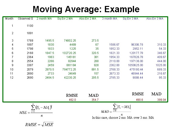
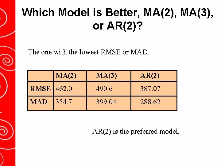
Moving Average: Example Month Observed S 1 1100 2 1891 3 4 5 6 7 8 9 10 11 12 1769 1897 1798 2168 2364 2554 3387 2079 2890 2690 2 month MA 1495. 5 1830 1833 1847. 5 1983 2266 2459 2970. 5 2733 2484. 5 Sq Err 2 MA Abs Err 2 MA 74802. 25 4489 1225 102720. 25 145161 82944 861184 794772. 25 24649 42230. 25 273. 5 67 35 320. 5 381 288 928 891. 5 157 205. 5 RMSE 462. 0 3 month MA 1586. 67 1852. 33 1821. 33 1954. 33 2110. 00 2362. 00 2768. 33 2673. 33 2785. 33 Sq Err 3 MA Abs Err 3 MA 96306. 78 2952. 11 120177. 78 167826. 78 197136. 00 1050625. 00 475180. 44 46944. 44 9088. 44 310. 33 54. 33 346. 67 409. 67 444. 00 1025. 00 689. 33 216. 67 95. 33 MAD RMSE MADMAD 354. 7 490. 6 399. 04 In this case, choose 2 mo. MA over 3 mo. MA

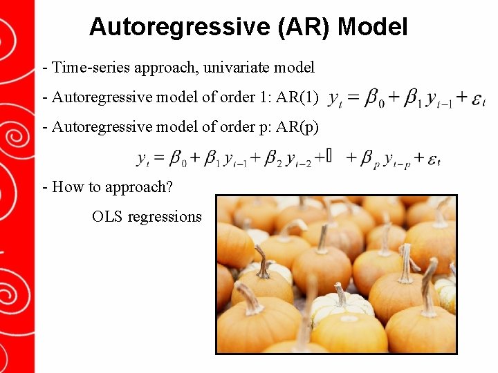
Autoregressive (AR) Model - Time-series approach, univariate model - Autoregressive model of order 1: AR(1) - Autoregressive model of order p: AR(p) - How to approach? OLS regressions

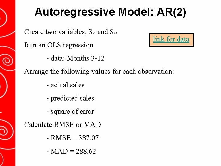
Autoregressive Model: AR(2) Create two variables, S and S t-1 Run an OLS regression t-2 link for data - data: Months 3 -12 Arrange the following values for each observation: - actual sales - predicted sales - square of error Calculate RMSE or MAD - RMSE = 387. 07 - MAD = 288. 62

Which Model is Better, MA(2), MA(3), or AR(2)? The one with the lowest RMSE or MAD. MA(2) MA(3) AR(2) RMSE 462. 0 490. 6 387. 07 MAD 399. 04 288. 62 354. 7 AR(2) is the preferred model.