Flow Control 1 TCP Flow Control flow control

Flow Control 1

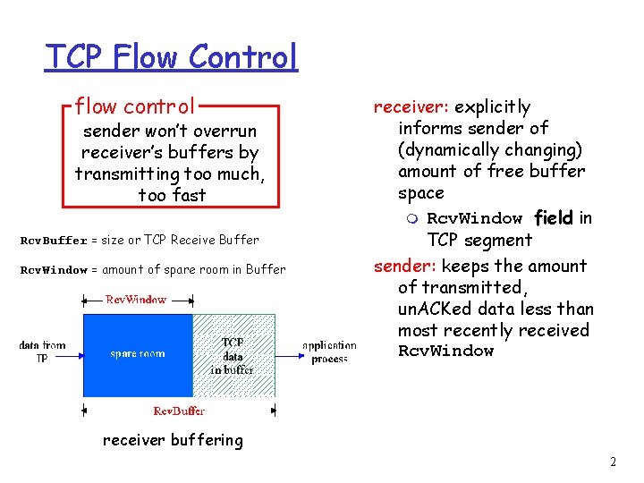
TCP Flow Control flow control sender won’t overrun receiver’s buffers by transmitting too much, too fast Rcv. Buffer = size or TCP Receive Buffer Rcv. Window = amount of spare room in Buffer receiver: explicitly informs sender of (dynamically changing) amount of free buffer space m Rcv. Window field in TCP segment sender: keeps the amount of transmitted, un. ACKed data less than most recently received Rcv. Window receiver buffering 2

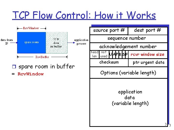
TCP Flow Control: How it Works source port # dest port # sequence number acknowledgement number head not len used U A P R S F r spare room in buffer = Rcv. Window checksum rcvr window size ptr urgent data Options (variable length) application data (variable length) 3 3

TCP: setting timeouts 4

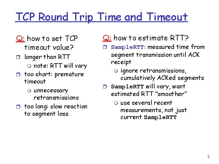
TCP Round Trip Time and Timeout Q: how to set TCP timeout value? r longer than RTT note: RTT will vary r too short: premature timeout m unnecessary retransmissions r too long: slow reaction to segment loss m Q: how to estimate RTT? r Sample. RTT: measured time from segment transmission until ACK receipt m ignore retransmissions, cumulatively ACKed segments r Sample. RTT will vary, want estimated RTT “smoother” m use several recent measurements, not just current Sample. RTT 5

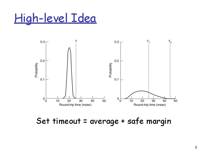
High-level Idea Set timeout = average + safe margin 6

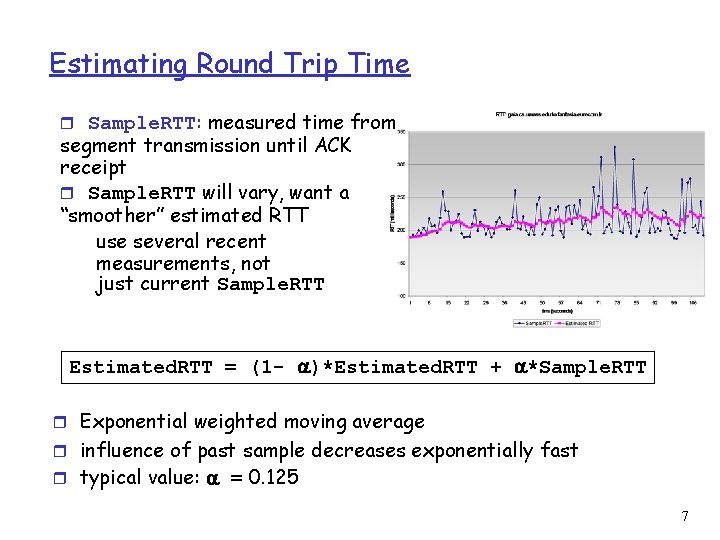
Estimating Round Trip Time r Sample. RTT: measured time from segment transmission until ACK receipt r Sample. RTT will vary, want a “smoother” estimated RTT use several recent measurements, not just current Sample. RTT Estimated. RTT = (1 - )*Estimated. RTT + *Sample. RTT r Exponential weighted moving average r influence of past sample decreases exponentially fast r typical value: = 0. 125 7

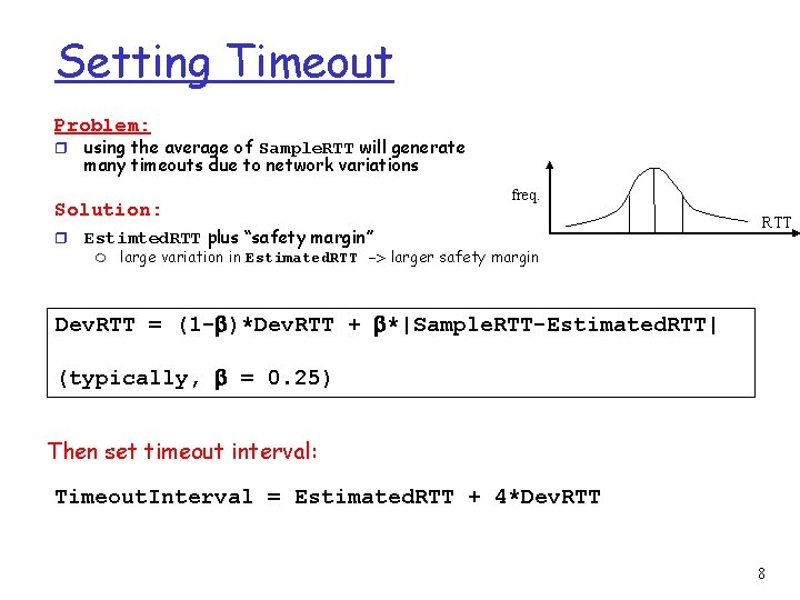
Setting Timeout Problem: r using the average of Sample. RTT will generate many timeouts due to network variations Solution: r freq. Estimted. RTT plus “safety margin” m RTT large variation in Estimated. RTT -> larger safety margin Dev. RTT = (1 - )*Dev. RTT + *|Sample. RTT-Estimated. RTT| (typically, = 0. 25) Then set timeout interval: Timeout. Interval = Estimated. RTT + 4*Dev. RTT 8

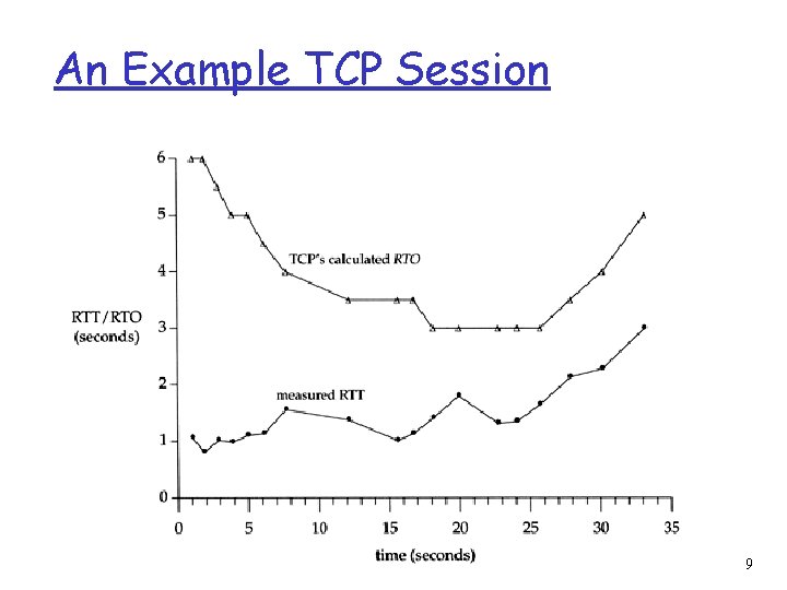
An Example TCP Session 9

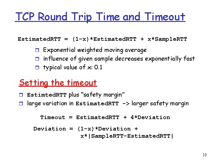
TCP Round Trip Time and Timeout Estimated. RTT = (1 -x)*Estimated. RTT + x*Sample. RTT r Exponential weighted moving average r influence of given sample decreases exponentially fast r typical value of x: 0. 1 Setting the timeout r Estimted. RTT plus “safety margin” r large variation in Estimated. RTT -> larger safety margin Timeout = Estimated. RTT + 4*Deviation = (1 -x)*Deviation + x*|Sample. RTT-Estimated. RTT| 10

Fast retransmit 11

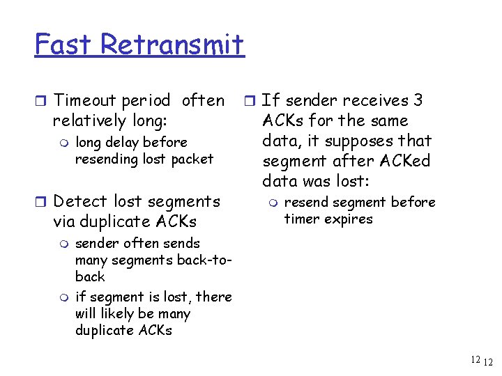
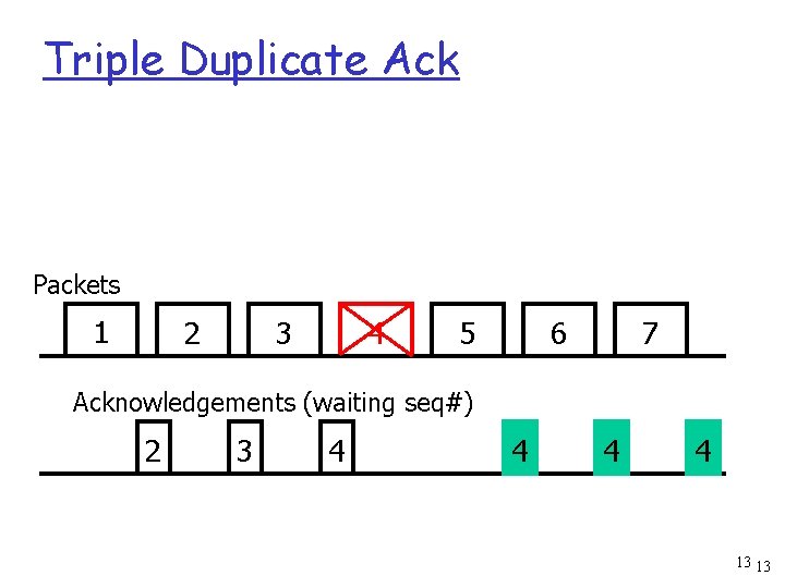
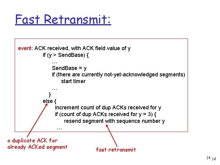
Fast Retransmit r Timeout period often relatively long: m long delay before resending lost packet r Detect lost segments via duplicate ACKs m m r If sender receives 3 ACKs for the same data, it supposes that segment after ACKed data was lost: m resend segment before timer expires sender often sends many segments back-toback if segment is lost, there will likely be many duplicate ACKs 12 12

Triple Duplicate Ack Packets 1 2 3 4 5 7 6 Acknowledgements (waiting seq#) 2 3 4 4 13 13

Fast Retransmit: event: ACK received, with ACK field value of y if (y > Send. Base) { … Send. Base = y if (there are currently not-yet-acknowledged segments) start timer … } else { increment count of dup ACKs received for y if (count of dup ACKs received for y = 3) { resend segment with sequence number y … a duplicate ACK for already ACKed segment fast retransmit 14 14

Congestion Control 15

Principles of Congestion Control Congestion: r informally: “too many sources sending too much data too fast for network to handle” r manifestations: m lost packets (buffer overflow at routers) m long delays (queuing in router buffers) r a highly important problem! 16

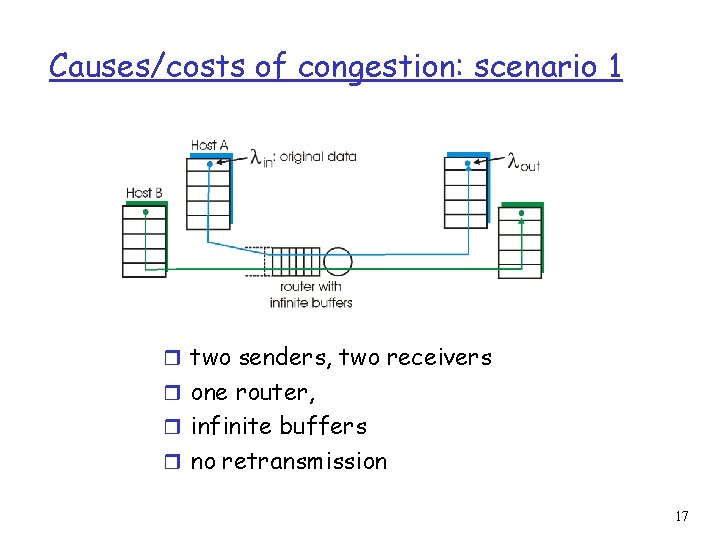
Causes/costs of congestion: scenario 1 r two senders, two receivers r one router, r infinite buffers r no retransmission 17

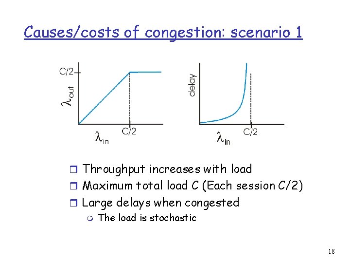
Causes/costs of congestion: scenario 1 r Throughput increases with load r Maximum total load C (Each session C/2) r Large delays when congested m The load is stochastic 18

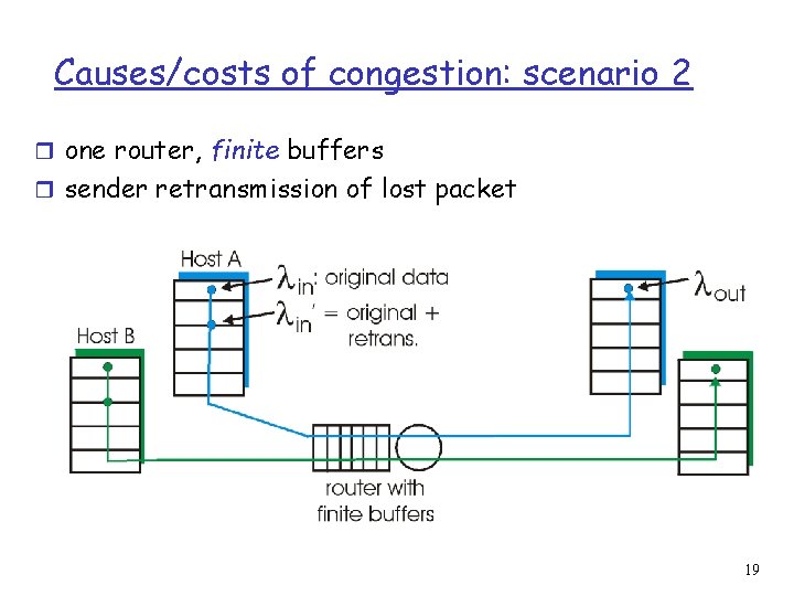
Causes/costs of congestion: scenario 2 r one router, finite buffers r sender retransmission of lost packet 19

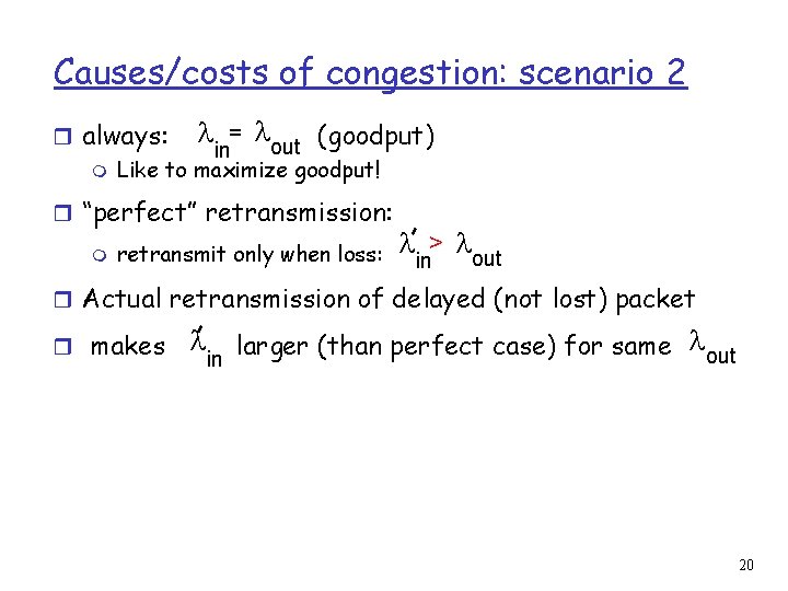
Causes/costs of congestion: scenario 2 r always: = out (goodput) in m Like to maximize goodput! r “perfect” retransmission: m retransmit only when loss: > out in r Actual retransmission of delayed (not lost) packet r makes larger (than perfect case) for same out in 20

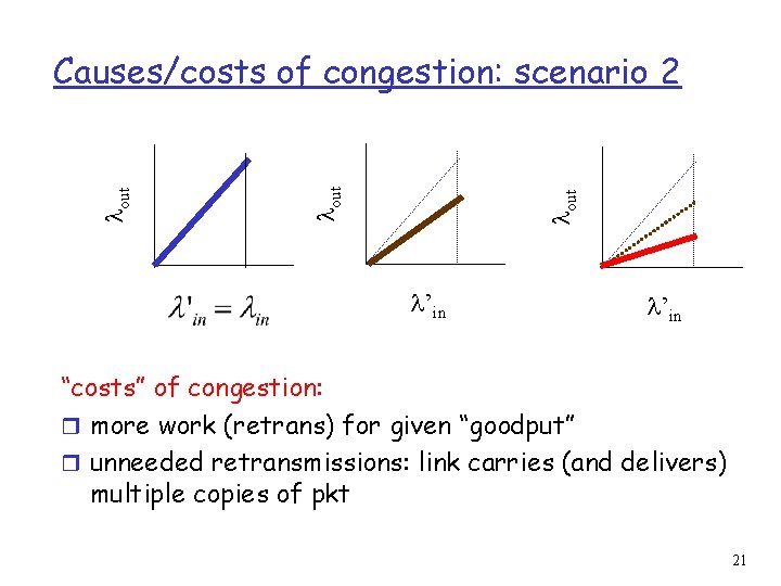
out Causes/costs of congestion: scenario 2 ’in “costs” of congestion: r more work (retrans) for given “goodput” r unneeded retransmissions: link carries (and delivers) multiple copies of pkt 21

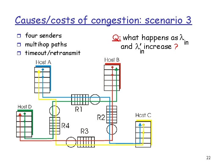
Causes/costs of congestion: scenario 3 r four senders r multihop paths r timeout/retransmit Q: what happens as in and increase ? in 22

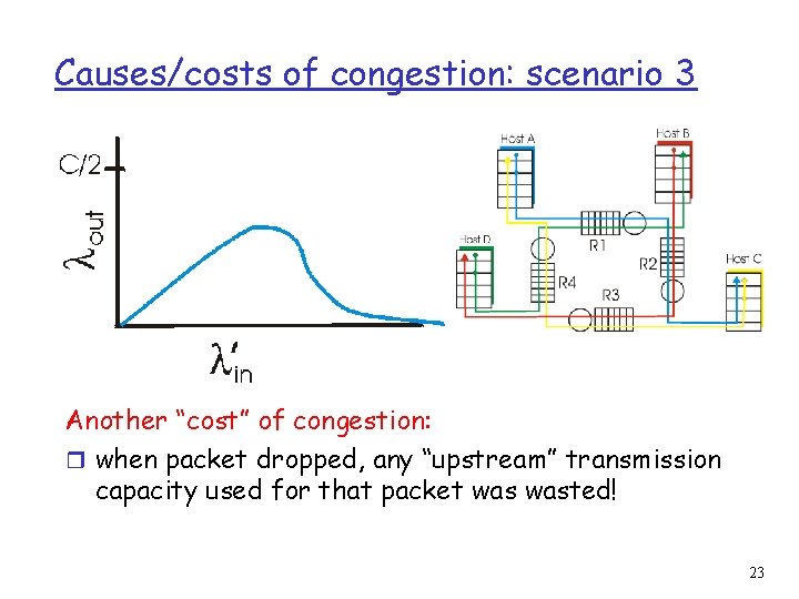
Causes/costs of congestion: scenario 3 Another “cost” of congestion: r when packet dropped, any “upstream” transmission capacity used for that packet wasted! 23

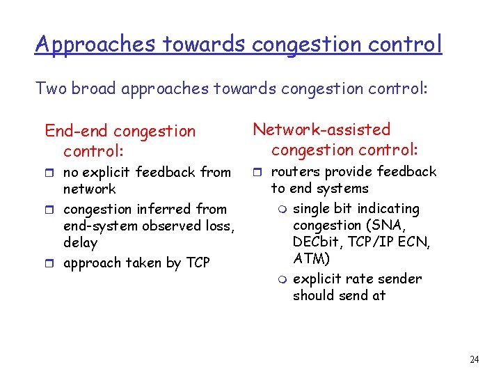
Approaches towards congestion control Two broad approaches towards congestion control: End-end congestion control: r no explicit feedback from network r congestion inferred from end-system observed loss, delay r approach taken by TCP Network-assisted congestion control: r routers provide feedback to end systems m single bit indicating congestion (SNA, DECbit, TCP/IP ECN, ATM) m explicit rate sender should send at 24

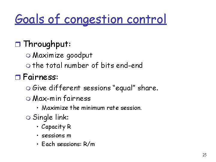
Goals of congestion control r Throughput: m Maximize goodput m the total number of bits end-end r Fairness: m Give different sessions “equal” share. m Max-min fairness • Maximize the minimum rate session. m Single link: • Capacity R • sessions m • Each sessions: R/m 25

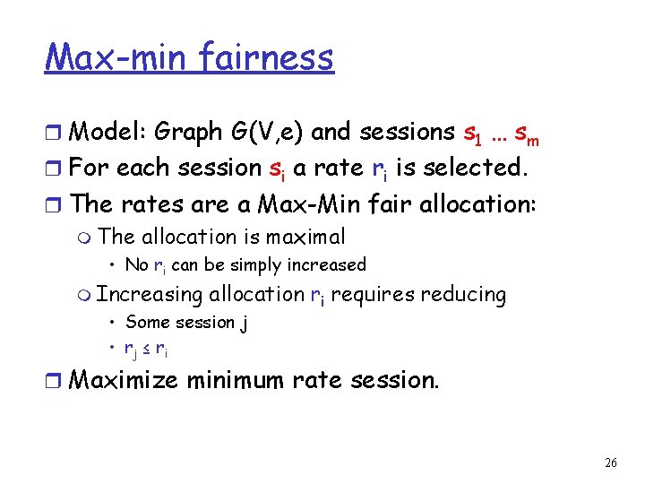
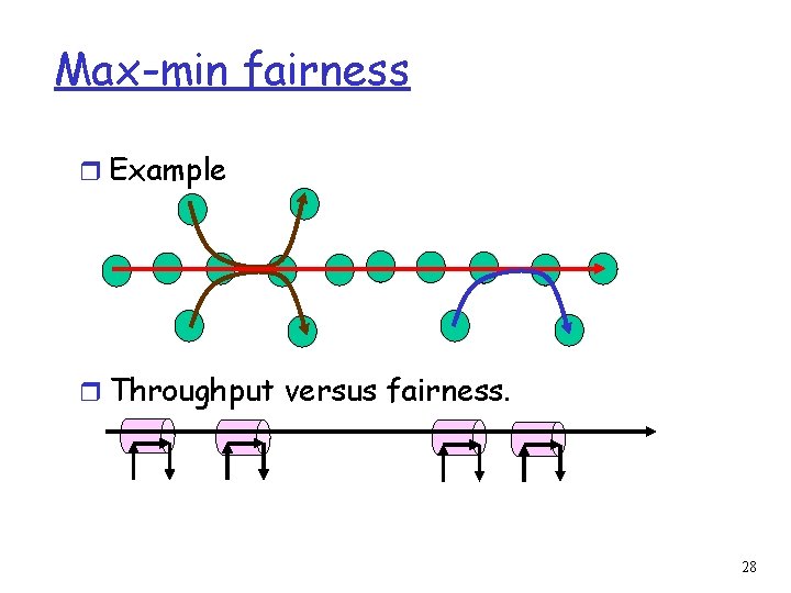
Max-min fairness r Model: Graph G(V, e) and sessions s 1 … sm r For each session si a rate ri is selected. r The rates are a Max-Min fair allocation: m The allocation is maximal • No ri can be simply increased m Increasing allocation ri requires reducing • Some session j • rj ≤ ri r Maximize minimum rate session. 26

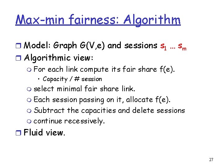
Max-min fairness: Algorithm r Model: Graph G(V, e) and sessions s 1 … sm r Algorithmic view: m For each link compute its fair share f(e). • Capacity / # session m select minimal fair share link. m Each session passing on it, allocate f(e). m Subtract the capacities and delete sessions m continue recessively. r Fluid view. 27

Max-min fairness r Example r Throughput versus fairness. 28

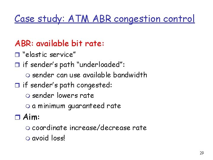
Case study: ATM ABR congestion control ABR: available bit rate: r “elastic service” r if sender’s path “underloaded”: m sender can use available bandwidth r if sender’s path congested: m sender lowers rate m a minimum guaranteed rate r Aim: m coordinate increase/decrease rate m avoid loss! 29

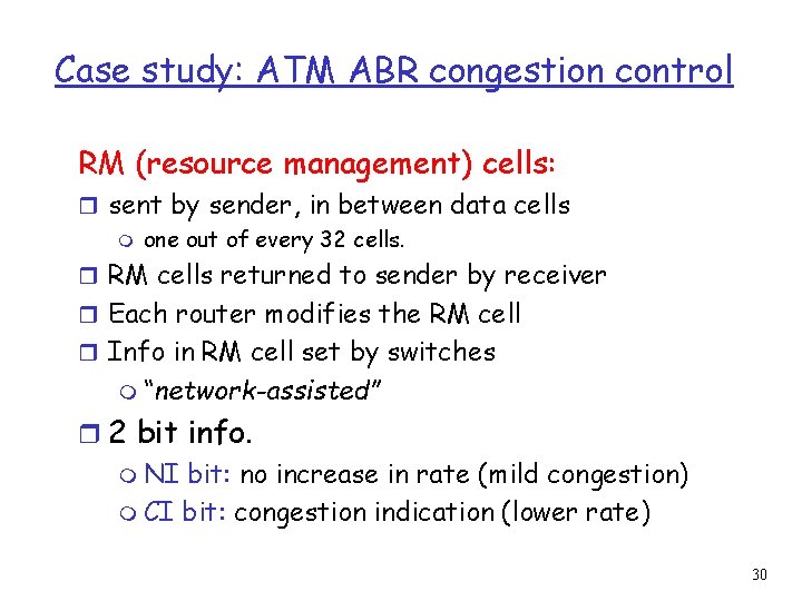
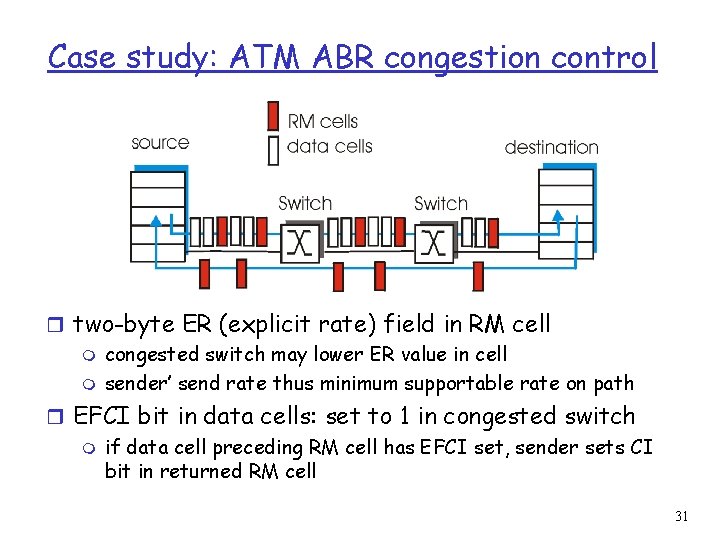
Case study: ATM ABR congestion control RM (resource management) cells: r sent by sender, in between data cells m one out of every 32 cells. r RM cells returned to sender by receiver r Each router modifies the RM cell r Info in RM cell set by switches m “network-assisted” r 2 bit info. m NI bit: no increase in rate (mild congestion) m CI bit: congestion indication (lower rate) 30

Case study: ATM ABR congestion control r two-byte ER (explicit rate) field in RM cell m congested switch may lower ER value in cell m sender’ send rate thus minimum supportable rate on path r EFCI bit in data cells: set to 1 in congested switch m if data cell preceding RM cell has EFCI set, sender sets CI bit in returned RM cell 31

Case study: ATM ABR congestion control r How does the router selects its action: m selects a rate m Set congestion bits m Vendor dependent functionality r Advantages: m fast response m accurate response r Disadvantages: m network level design m Increase router tasks (load). m Interoperability issues. 32

End to end control 33

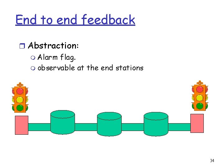
End to end feedback r Abstraction: m Alarm flag. m observable at the end stations 34

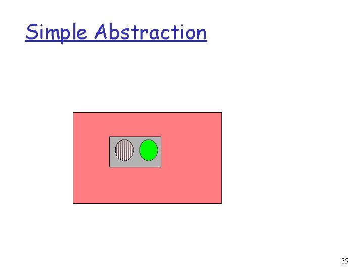
Simple Abstraction 35

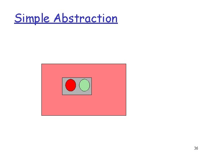
Simple Abstraction 36

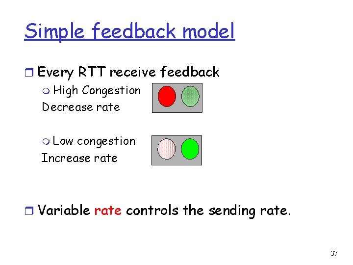
Simple feedback model r Every RTT receive feedback m High Congestion Decrease rate m Low congestion Increase rate r Variable rate controls the sending rate. 37

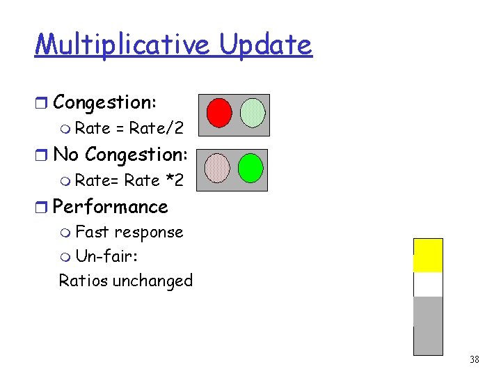
Multiplicative Update r Congestion: m Rate = Rate/2 r No Congestion: m Rate= Rate *2 r Performance m Fast response m Un-fair: Ratios unchanged 38

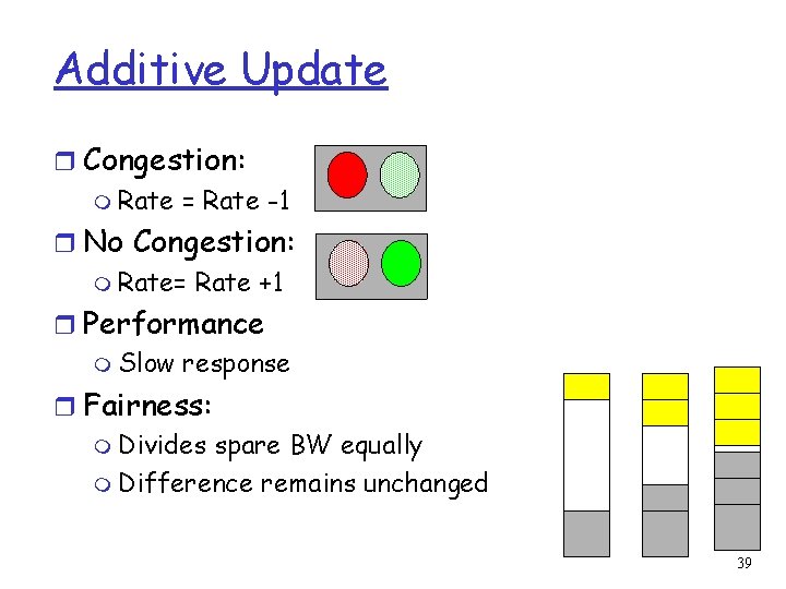
Additive Update r Congestion: m Rate = Rate -1 r No Congestion: m Rate= Rate +1 r Performance m Slow response r Fairness: m Divides spare BW equally m Difference remains unchanged 39

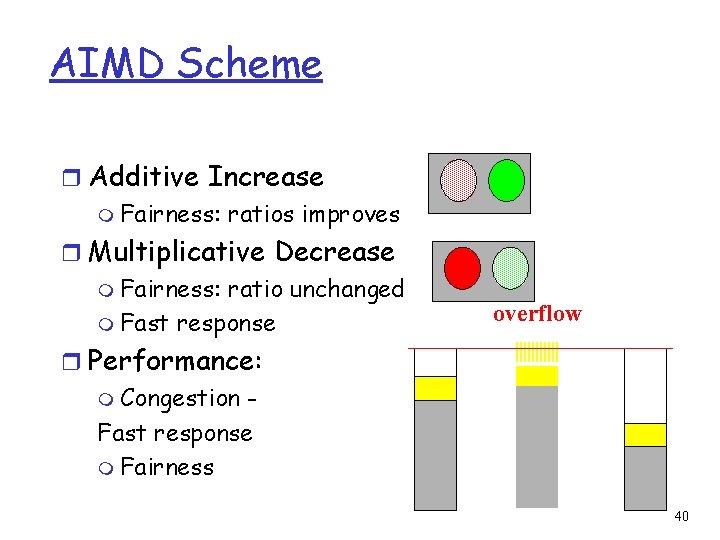
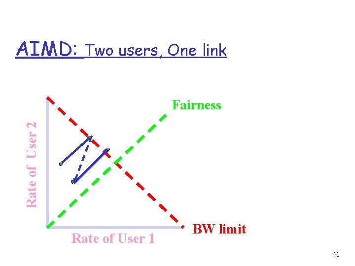
AIMD Scheme r Additive Increase m Fairness: ratios improves r Multiplicative Decrease m Fairness: ratio unchanged m Fast response overflow r Performance: m Congestion Fast response m Fairness 40

AIMD: Two users, One link Rate of User 2 Fairness Rate of User 1 BW limit 41

TCP Congestion Control r Closed-loop, end-to-end, window-based congestion control r Designed by Van Jacobson in late 1980 s, based on the AIMD alg. of Dah-Ming Chu and Raj Jain r Works well so far: the bandwidth of the Internet has increased by more than 200, 000 times r Many versions m TCP/Tahoe: this is a less optimized version m TCP/Reno: many OSs today implement Reno type congestion control m TCP/Vegas: not currently used For more details: see TCP/IP illustrated; or read http: //lxr. linux. no/source/net/ipv 4/tcp_input. c for linux implementation 42 42

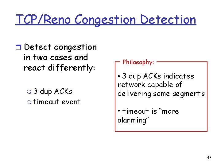
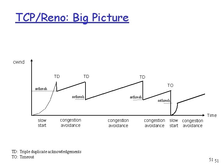
TCP/Reno Congestion Detection r Detect congestion in two cases and react differently: m 3 dup ACKs m timeout event Philosophy: • 3 dup ACKs indicates network capable of delivering some segments • timeout is “more alarming” 43

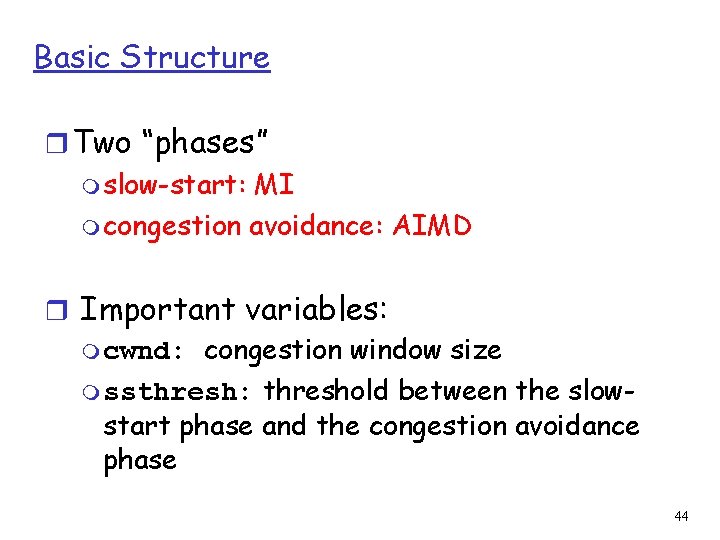
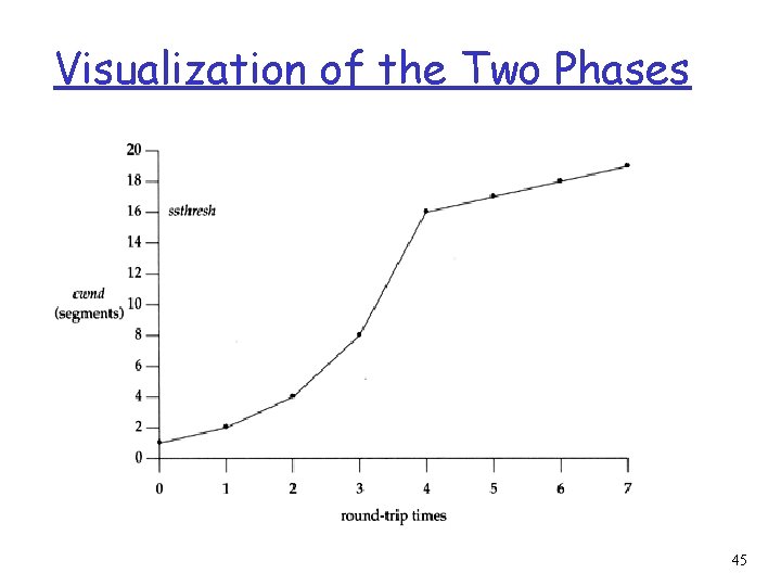
Basic Structure r Two “phases” m slow-start: MI m congestion avoidance: AIMD r Important variables: m cwnd: congestion window size m ssthresh: threshold between the slowstart phase and the congestion avoidance phase 44

Visualization of the Two Phases 45

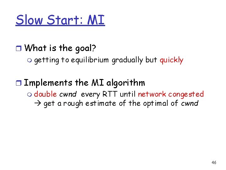
Slow Start: MI r What is the goal? m getting to equilibrium gradually but quickly r Implements the MI algorithm m double cwnd every RTT until network congested get a rough estimate of the optimal of cwnd 46

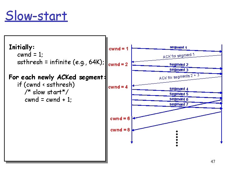
Slow-start Initially: cwnd = 1; ssthresh = infinite (e. g. , 64 K); For each newly ACKed segment: if (cwnd < ssthresh) /* slow start*/ cwnd = cwnd + 1; cwnd = 1 segment 1 ACK for segm cwnd = 2 ent 1 segment 2 segment 3 ents 2 + 3 ACK for segm cwnd = 4 segment 5 segment 6 segment 7 cwnd = 6 cwnd = 8 47

Startup Behavior with Slow-start See [Jac 89] 48

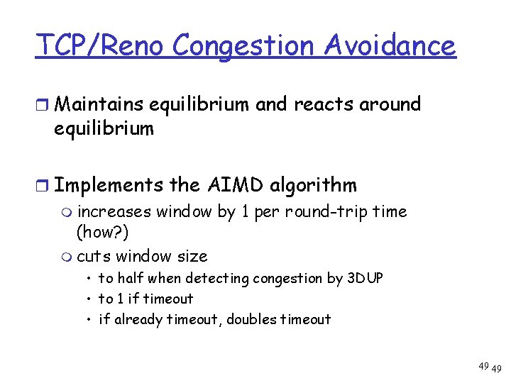
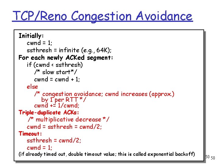
TCP/Reno Congestion Avoidance r Maintains equilibrium and reacts around equilibrium r Implements the AIMD algorithm m increases window by 1 per round-trip time (how? ) m cuts window size • to half when detecting congestion by 3 DUP • to 1 if timeout • if already timeout, doubles timeout 49 49

TCP/Reno Congestion Avoidance Initially: cwnd = 1; ssthresh = infinite (e. g. , 64 K); For each newly ACKed segment: if (cwnd < ssthresh) /* slow start*/ cwnd = cwnd + 1; else /* congestion avoidance; cwnd increases (approx. ) by 1 per RTT */ cwnd += 1/cwnd; Triple-duplicate ACKs: /* multiplicative decrease */ cwnd = ssthresh = cwnd/2; Timeout: ssthresh = cwnd/2; cwnd = 1; (if already timed out, double timeout value; this is called exponential backoff) 50 50

TCP/Reno: Big Picture cwnd TD TD TD TO ssthresh Time slow start congestion avoidance TD: Triple duplicate acknowledgements TO: Timeout congestion avoidance slow congestion start avoidance 51 51

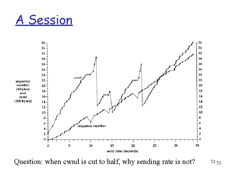
A Session Question: when cwnd is cut to half, why sending rate is not? 52 52

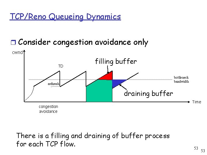
TCP/Reno Queueing Dynamics r Consider congestion avoidance only cwnd TD filling buffer bottleneck bandwidth ssthresh draining buffer Time congestion avoidance There is a filling and draining of buffer process for each TCP flow. 53 53

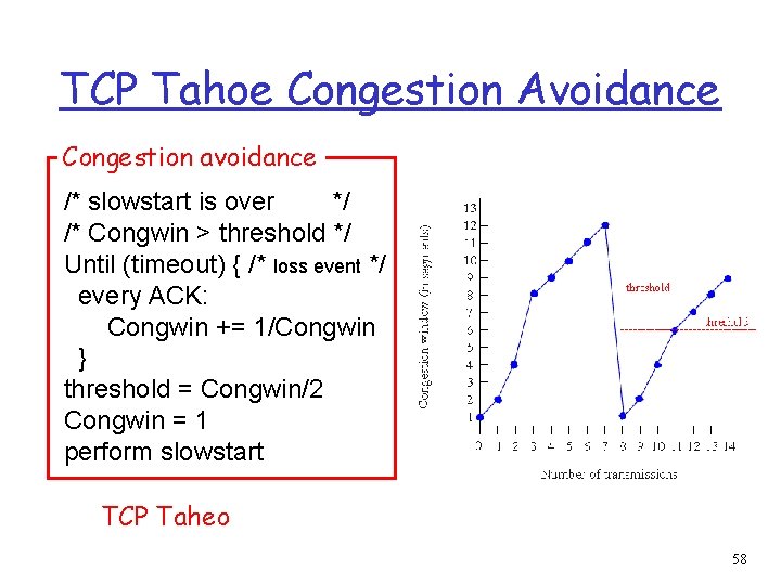
TCP Tahoe Congestion Avoidance Congestion avoidance /* slowstart is over */ /* Congwin > threshold */ Until (timeout) { /* loss event */ every ACK: Congwin += 1/Congwin } threshold = Congwin/2 Congwin = 1 perform slowstart TCP Taheo 58

TCP Reno r Fast retransmit: m After receiving 3 duplicate ACK m Resend first packet in window. • Try to avoid waiting for timeout r Fast recovery: m After retransmission do not enter slowstart. m Threshold = Congwin/2 m Congwin = 3 + Congwin/2 m Each duplicate ACK received Congwin++ m After new ACK • Congwin = Threshold • return to congestion avoidance r Single packet drop: great! 59

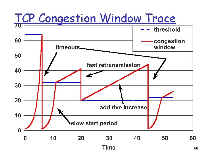
TCP Congestion Window Trace 60

TCP Vegas: r Idea: track the RTT m Try to avoid packet loss m latency increases: lower rate m latency very low: increase rate r Implementation: m sample_RTT: current RTT m Base_RTT: min. over sample_RTT m Expected = Congwin / Base_RTT m Actual = number of packets sent / sample_RTT m =Expected - Actual 61

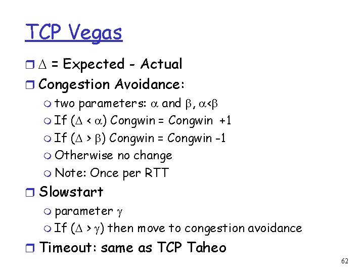
TCP Vegas r = Expected - Actual r Congestion Avoidance: m two parameters: and , < m If ( < ) Congwin = Congwin +1 m If ( > ) Congwin = Congwin -1 m Otherwise no change m Note: Once per RTT r Slowstart m parameter m If ( > ) then move to congestion avoidance r Timeout: same as TCP Taheo 62

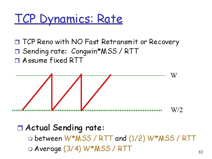
TCP Dynamics: Rate r TCP Reno with NO Fast Retransmit or Recovery r Sending rate: Congwin*MSS / RTT r Assume fixed RTT W W/2 r Actual Sending rate: m between W*MSS / RTT and (1/2) W*MSS / RTT m Average (3/4) W*MSS / RTT 63

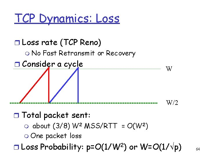
TCP Dynamics: Loss rate (TCP Reno) m No Fast Retransmit or Recovery r Consider a cycle W W/2 r Total packet sent: m about (3/8) W 2 MSS/RTT = O(W 2) m One packet loss r Loss Probability: p=O(1/W 2) or W=O(1/ p) 64

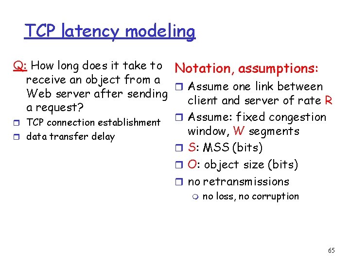
TCP latency modeling Q: How long does it take to Notation, assumptions: receive an object from a r Assume one link between Web server after sending client and server of rate R a request? r Assume: fixed congestion r TCP connection establishment window, W segments r data transfer delay r S: MSS (bits) r O: object size (bits) r no retransmissions m no loss, no corruption 65

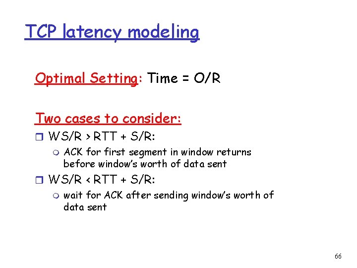
TCP latency modeling Optimal Setting: Time = O/R Two cases to consider: r WS/R > RTT + S/R: m ACK for first segment in window returns before window’s worth of data sent r WS/R < RTT + S/R: m wait for ACK after sending window’s worth of data sent 66

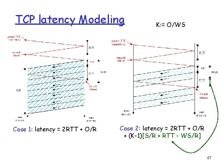
TCP latency Modeling Case 1: latency = 2 RTT + O/R K: = O/WS Case 2: latency = 2 RTT + O/R + (K-1)[S/R + RTT - WS/R] 67

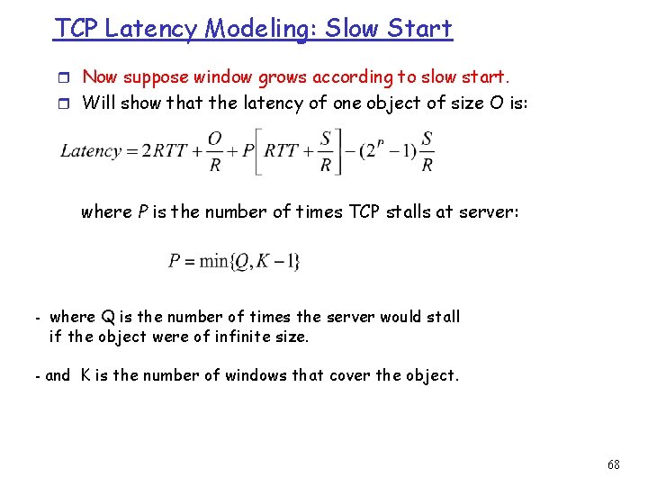
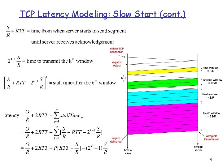
TCP Latency Modeling: Slow Start r Now suppose window grows according to slow start. r Will show that the latency of one object of size O is: where P is the number of times TCP stalls at server: - where Q is the number of times the server would stall if the object were of infinite size. - and K is the number of windows that cover the object. 68

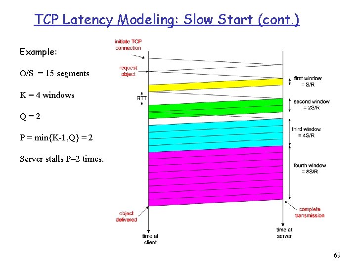
TCP Latency Modeling: Slow Start (cont. ) Example: O/S = 15 segments K = 4 windows Q=2 P = min{K-1, Q} = 2 Server stalls P=2 times. 69

TCP Latency Modeling: Slow Start (cont. ) 70