Fin 501 Asset Pricing Lecture 03 Risk Preferences

Fin 501: Asset Pricing Lecture 03: Risk Preferences and Expected Utility Theory • Prof. Markus K. Brunnermeier Lecture 03 Risk Aversion

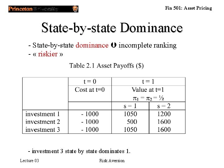
Fin 501: Asset Pricing State-by-state Dominance - State-by-state dominance incomplete ranking - « riskier » - investment 3 state by state dominates 1. Lecture 03 Risk Aversion

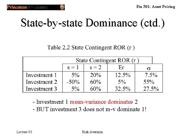
Fin 501: Asset Pricing State-by-state Dominance (ctd. ) - Investment 1 mean-variance dominates 2 - BUT investment 3 does not m-v dominate 1! Lecture 03 Risk Aversion

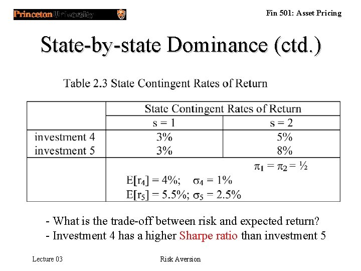
Fin 501: Asset Pricing State-by-state Dominance (ctd. ) - What is the trade-off between risk and expected return? - Investment 4 has a higher Sharpe ratio than investment 5 Lecture 03 Risk Aversion

Fin 501: Asset Pricing Stochastic Dominance • Stochastic dominance can be defined independently of the specific trade-offs (between return, risk and other characteristics of probability distributions) represented by an agent's utility function. (“risk-preference-free”) • Less “demanding” than state-by-state dominance Lecture 03 Risk Aversion

Fin 501: Asset Pricing Stochastic Dominance • Still incomplete ordering – “More complete” than state-by-state ordering – State-by-state dominance ) stochastic dominance – Risk preference not needed for ranking! • independently of the specific trade-offs (between return, risk and other characteristics of probability distributions) represented by an agent's utility function. (“risk-preference-free”) • Next Section: – Complete preference ordering and utility representations Homework: Provide an example which can be ranked according to FSD , but not according to state dominance. Lecture 03 Risk Aversion

Fin 501: Asset Pricing Lecture 03 Risk Aversion

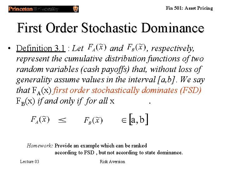
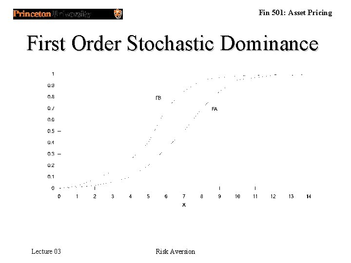
Fin 501: Asset Pricing First Order Stochastic Dominance • Definition 3. 1 : Let and , respectively, represent the cumulative distribution functions of two random variables (cash payoffs) that, without loss of generality assume values in the interval [a, b]. We say that FA(x) first order stochastically dominates (FSD) FB(x) if and only if for all x. Homework: Provide an example which can be ranked according to FSD , but not according to state dominance. Lecture 03 Risk Aversion

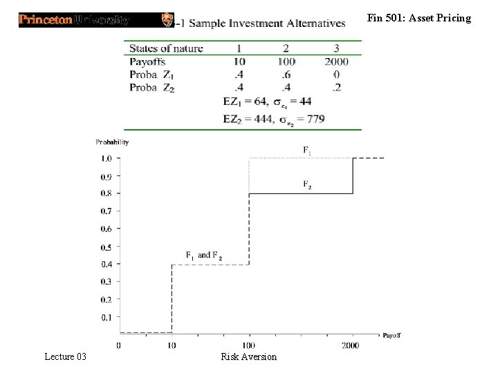
Fin 501: Asset Pricing First Order Stochastic Dominance Lecture 03 Risk Aversion

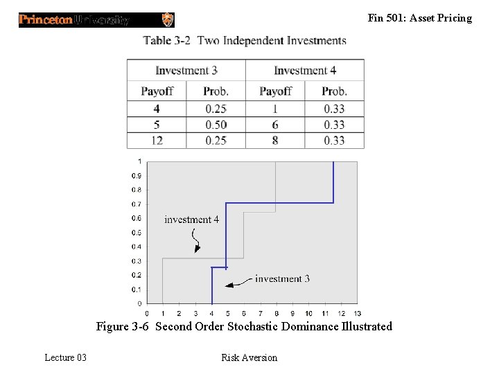
Fin 501: Asset Pricing Figure 3 -6 Second Order Stochastic Dominance Illustrated Lecture 03 Risk Aversion

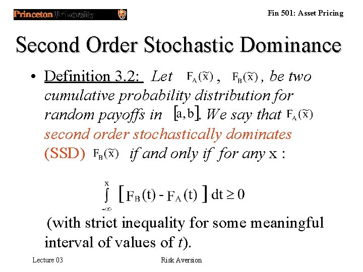
Fin 501: Asset Pricing Second Order Stochastic Dominance • Definition 3. 2: Let , , be two cumulative probability distribution for random payoffs in. We say that second order stochastically dominates (SSD) if and only if for any x : (with strict inequality for some meaningful interval of values of t). Lecture 03 Risk Aversion

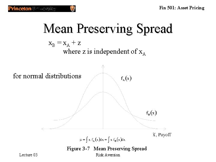
Fin 501: Asset Pricing Mean Preserving Spread x. B = x. A + z where z is independent of x. A for normal distributions Figure 3 -7 Mean Preserving Spread Lecture 03 Risk Aversion

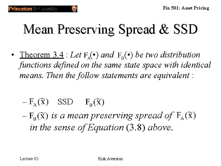
Fin 501: Asset Pricing Mean Preserving Spread & SSD • Theorem 3. 4 : Let ( • ) and ( • ) be two distribution functions defined on the same state space with identical means. Then the follow statements are equivalent : – SSD is a mean preserving spread of in the sense of Equation (3. 8) above. – Lecture 03 Risk Aversion

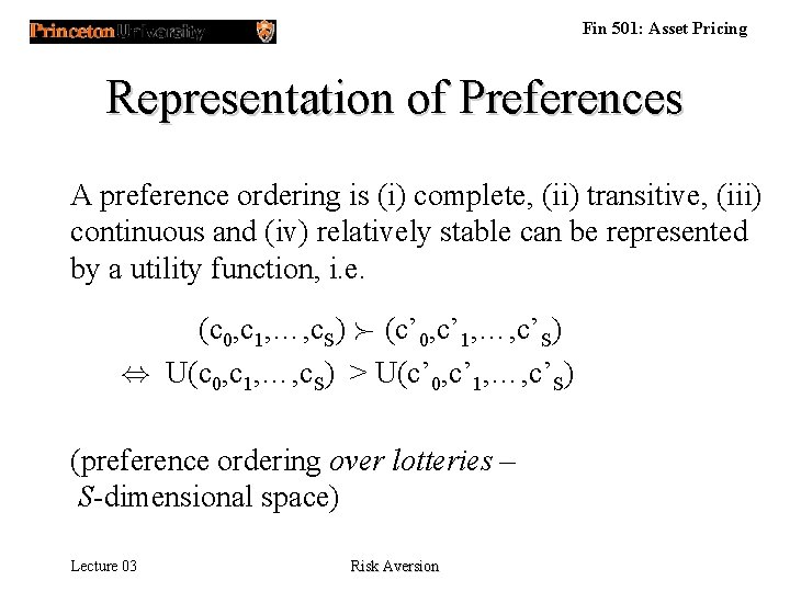
Fin 501: Asset Pricing Representation of Preferences A preference ordering is (i) complete, (ii) transitive, (iii) continuous and (iv) relatively stable can be represented by a utility function, i. e. (c 0, c 1, …, c. S) (c’ 0, c’ 1, …, c’S) , U(c 0, c 1, …, c. S) > U(c’ 0, c’ 1, …, c’S) (preference ordering over lotteries – S-dimensional space) Lecture 03 Risk Aversion

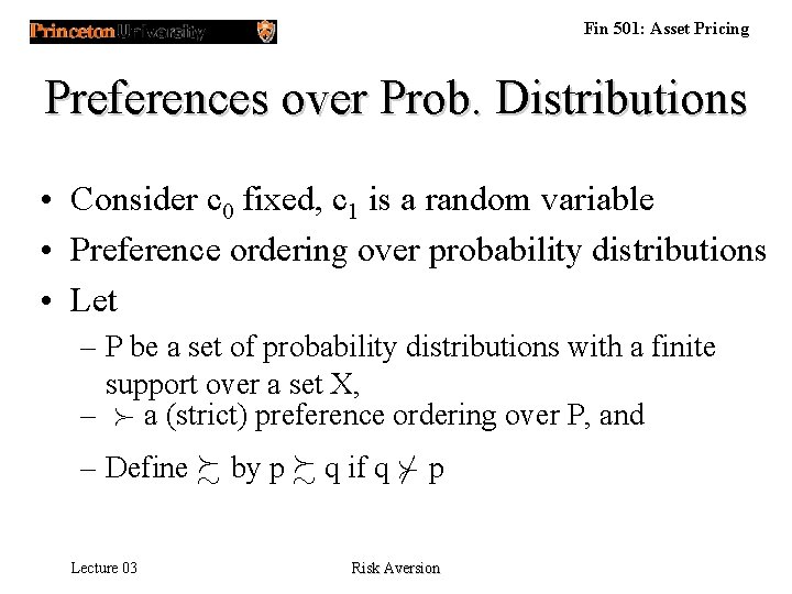
Fin 501: Asset Pricing Preferences over Prob. Distributions • Consider c 0 fixed, c 1 is a random variable • Preference ordering over probability distributions • Let – P be a set of probability distributions with a finite support over a set X, – a (strict) preference ordering over P, and – Define % by p % q if q ¨ p Lecture 03 Risk Aversion

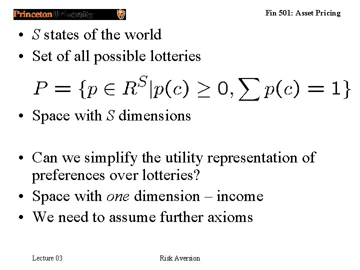
Fin 501: Asset Pricing • S states of the world • Set of all possible lotteries • Space with S dimensions • Can we simplify the utility representation of preferences over lotteries? • Space with one dimension – income • We need to assume further axioms Lecture 03 Risk Aversion

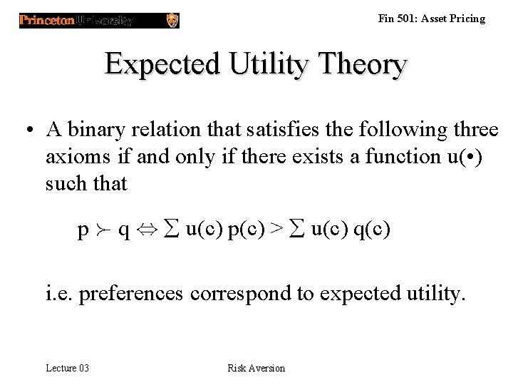
Fin 501: Asset Pricing Expected Utility Theory • A binary relation that satisfies the following three axioms if and only if there exists a function u( • ) such that p q , å u(c) p(c) > å u(c) q(c) i. e. preferences correspond to expected utility. Lecture 03 Risk Aversion

Fin 501: Asset Pricing Expected Utility Theory Lecture 03 Risk Aversion

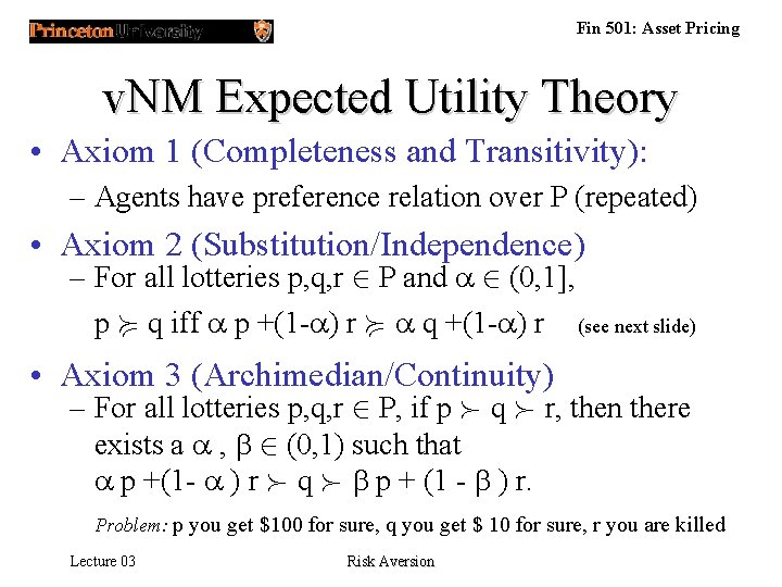
Fin 501: Asset Pricing v. NM Expected Utility Theory • Axiom 1 (Completeness and Transitivity): – Agents have preference relation over P (repeated) • Axiom 2 (Substitution/Independence) – For all lotteries p, q, r 2 P and a 2 (0, 1], p < q iff a p +(1 -a) r < a q +(1 -a) r (see next slide) • Axiom 3 (Archimedian/Continuity) – For all lotteries p, q, r 2 P, if p q r, then there exists a a , b 2 (0, 1) such that a p +(1 - a ) r q b p + (1 - b ) r. Problem: p you get $100 for sure, q you get $ 10 for sure, r you are killed Lecture 03 Risk Aversion

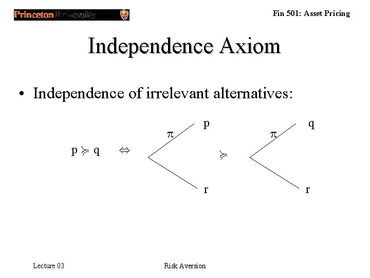
Fin 501: Asset Pricing Independence Axiom • Independence of irrelevant alternatives: p p p < q , < r Lecture 03 p q Risk Aversion r

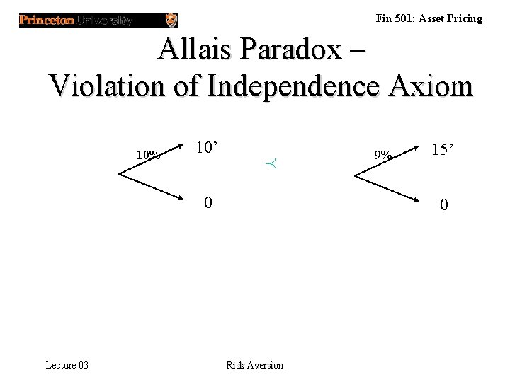
Fin 501: Asset Pricing Allais Paradox – Violation of Independence Axiom 10% 10’ Á 0 Lecture 03 9% 15’ 0 Risk Aversion

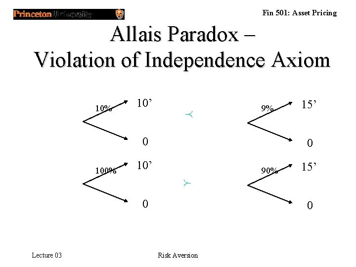
Fin 501: Asset Pricing Allais Paradox – Violation of Independence Axiom 10% 10’ Á 9% 0 100% Lecture 03 0 10’ 0 15’ 90% 15’ 0 Risk Aversion

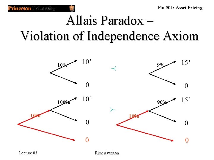
Fin 501: Asset Pricing Allais Paradox – Violation of Independence Axiom 10% 10’ 9% Á 0 100% 10% 0 10’ 0 90% 0 Lecture 03 15’ 10% 15’ 0 0 Risk Aversion

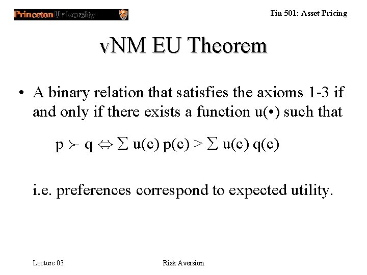
Fin 501: Asset Pricing v. NM EU Theorem • A binary relation that satisfies the axioms 1 -3 if and only if there exists a function u( • ) such that p q , å u(c) p(c) > å u(c) q(c) i. e. preferences correspond to expected utility. Lecture 03 Risk Aversion

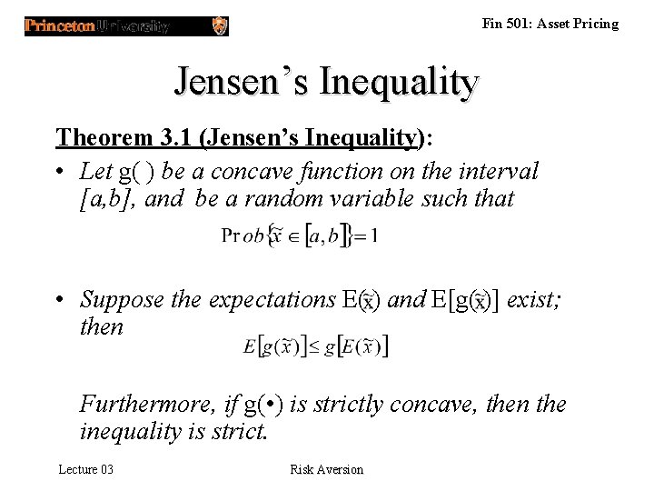
Fin 501: Asset Pricing Jensen’s Inequality Theorem 3. 1 (Jensen’s Inequality): • Let g( ) be a concave function on the interval [a, b], and be a random variable such that • Suppose the expectations E( ) and E[g( )] exist; then Furthermore, if g( • ) is strictly concave, then the inequality is strict. Lecture 03 Risk Aversion

Fin 501: Asset Pricing Expected Utility Theory Lecture 03 Risk Aversion

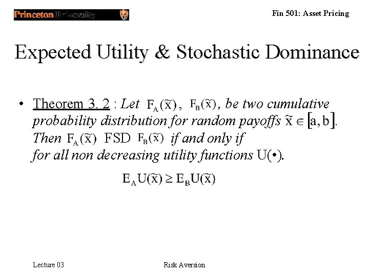
Fin 501: Asset Pricing Expected Utility & Stochastic Dominance • Theorem 3. 2 : Let , , be two cumulative probability distribution for random payoffs. Then FSD if and only if for all non decreasing utility functions U( • ). Lecture 03 Risk Aversion

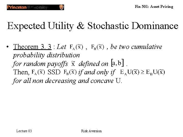
Fin 501: Asset Pricing Expected Utility & Stochastic Dominance • Theorem 3. 3 : Let , , be two cumulative probability distribution for random payoffs defined on. Then, SSD if and only if for all non decreasing and concave U. Lecture 03 Risk Aversion

Fin 501: Asset Pricing Digression: Subjective EU Theory • Derive perceived probability from preferences! – Set S of prizes/consequences – Set Z of states – Set of functions f(s) 2 Z, called acts (consumption plans) • Seven SAVAGE Axioms – Goes beyond scope of this course. Lecture 03 Risk Aversion

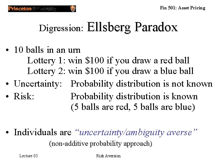
Fin 501: Asset Pricing Digression: Ellsberg Paradox • 10 balls in an urn Lottery 1: win $100 if you draw a red ball Lottery 2: win $100 if you draw a blue ball • Uncertainty: Probability distribution is not known • Risk: Probability distribution is known (5 balls are red, 5 balls are blue) • Individuals are “uncertainty/ambiguity averse” (non-additive probability approach) Lecture 03 Risk Aversion

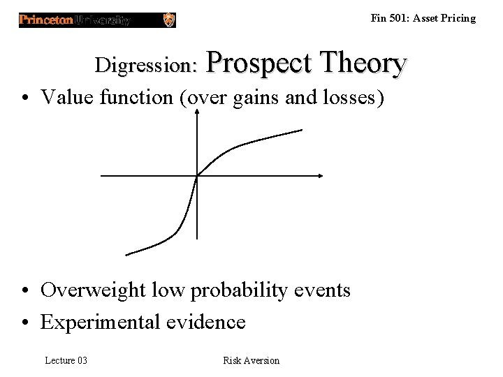
Fin 501: Asset Pricing Digression: Prospect Theory • Value function (over gains and losses) • Overweight low probability events • Experimental evidence Lecture 03 Risk Aversion

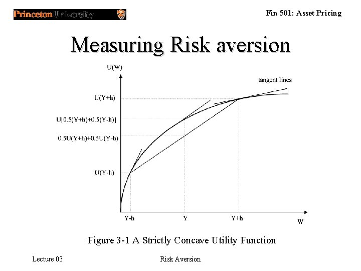
Fin 501: Asset Pricing Measuring Risk aversion Figure 3 -1 A Strictly Concave Utility Function Lecture 03 Risk Aversion

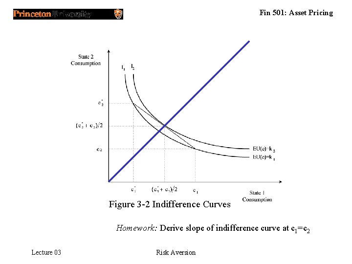
Fin 501: Asset Pricing Figure 3 -2 Indifference Curves Homework: Derive slope of indifference curve at c 1=c 2 Lecture 03 Risk Aversion

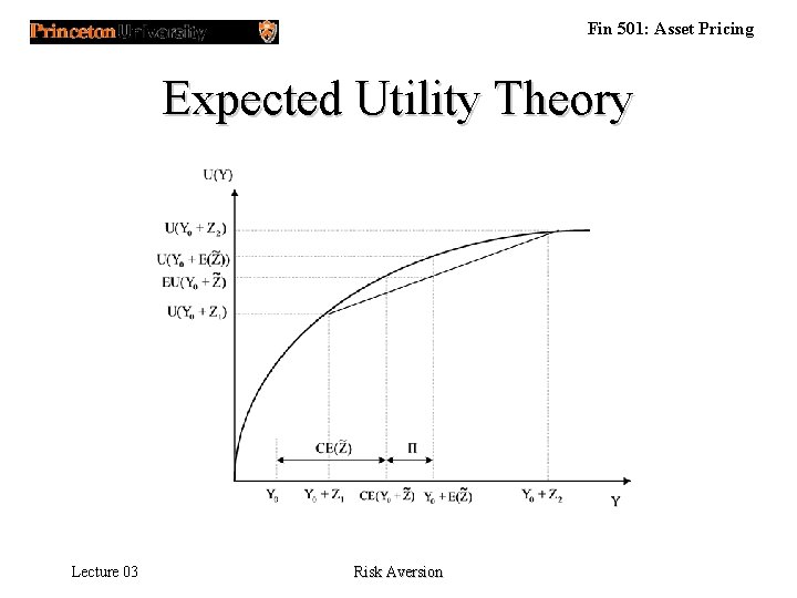
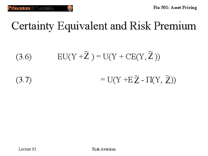
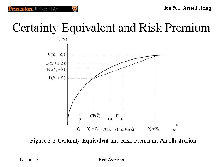
Fin 501: Asset Pricing Certainty Equivalent and Risk Premium (3. 6) (3. 7) Lecture 03 EU(Y + ) = U(Y + CE(Y, )) = U(Y +E - (Y, )) Risk Aversion

Fin 501: Asset Pricing Certainty Equivalent and Risk Premium Figure 3 -3 Certainty Equivalent and Risk Premium: An Illustration Lecture 03 Risk Aversion

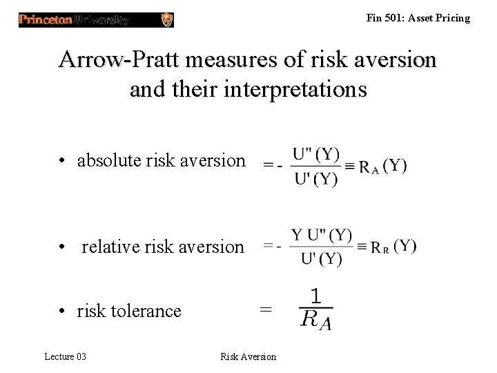
Fin 501: Asset Pricing Arrow-Pratt measures of risk aversion and their interpretations • absolute risk aversion • relative risk aversion • risk tolerance = Lecture 03 Risk Aversion

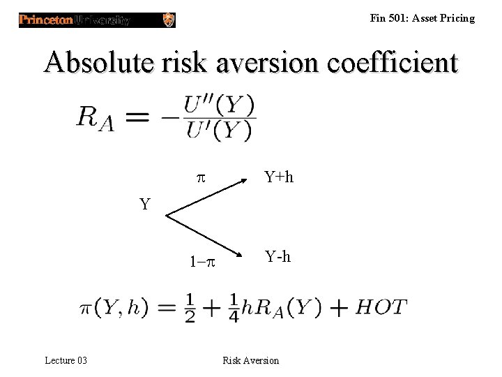
Fin 501: Asset Pricing Absolute risk aversion coefficient p Y+h 1 -p Y-h Y Lecture 03 Risk Aversion

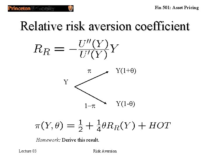
Fin 501: Asset Pricing Relative risk aversion coefficient p Y(1+q) 1 -p Y(1 -q) Y Homework: Derive this result. Lecture 03 Risk Aversion

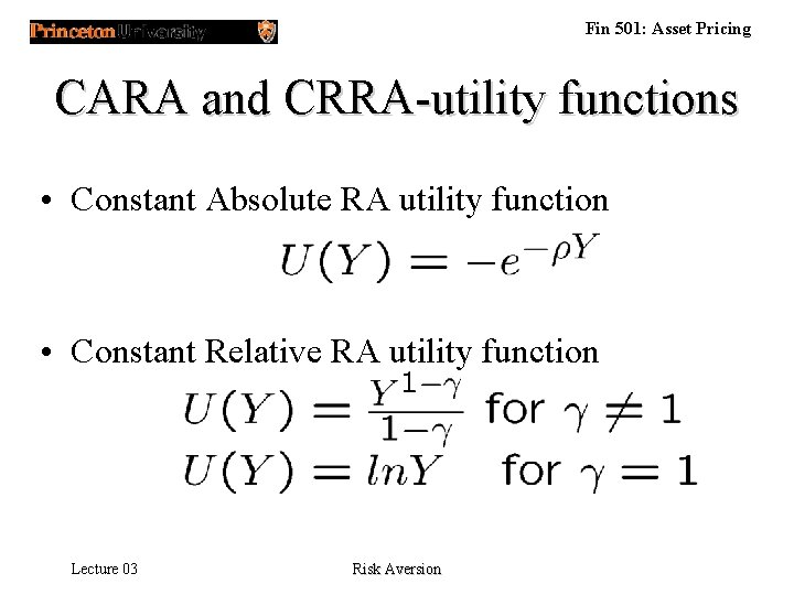
Fin 501: Asset Pricing CARA and CRRA-utility functions • Constant Absolute RA utility function • Constant Relative RA utility function Lecture 03 Risk Aversion

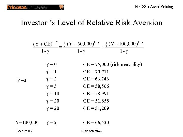
Fin 501: Asset Pricing Investor ’s Level of Relative Risk Aversion Y=0 = 1 = 2 = 5 = 10 = 20 = 30 CE = 75, 000 (risk neutrality) CE = 70, 711 CE = 66, 246 CE = 58, 566 CE = 53, 991 CE = 51, 858 CE = 51, 209 Y=100, 000 = 5 CE = 66, 530 Lecture 03 Risk Aversion

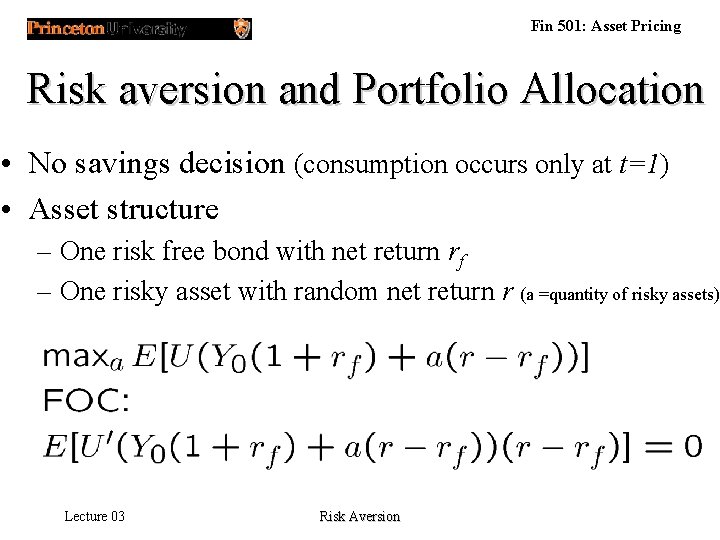
Fin 501: Asset Pricing Risk aversion and Portfolio Allocation • No savings decision (consumption occurs only at t=1) • Asset structure – One risk free bond with net return rf – One risky asset with random net return r (a =quantity of risky assets) Lecture 03 Risk Aversion

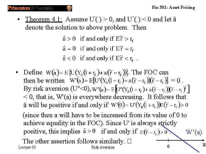
Fin 501: Asset Pricing • Theorem 4. 1: Assume U'( ) > 0, and U"( ) < 0 and let â denote the solution to above problem. Then • Define . The FOC can then be written = 0. By risk aversion (U''<0), < 0, that is, W'(a) is everywhere decreasing. It follows that â will be positive if and only if (since then a will have to be increased from its value of 0 to achieve equality in the FOC). Since U' is always strictly positive, this implies if and only if . W’(a) The other assertion follows similarly. � a Lecture 03 Risk Aversion 0

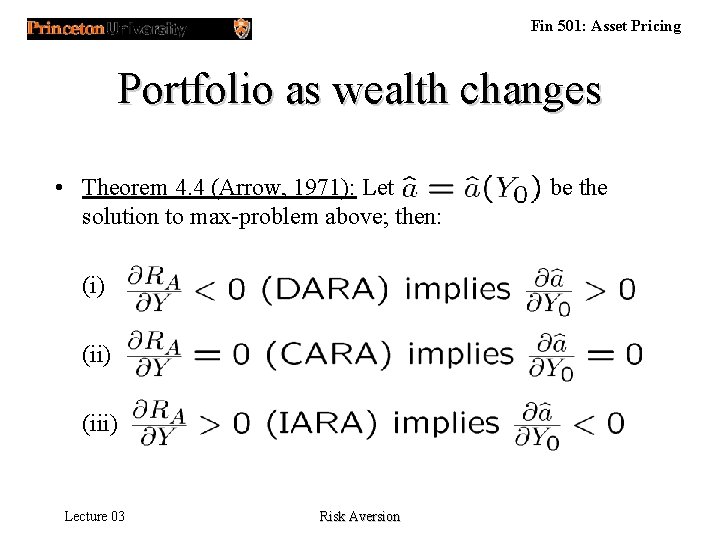
Fin 501: Asset Pricing Portfolio as wealth changes • Theorem 4. 4 (Arrow, 1971): Let be the solution to max-problem above; then: (i) (iii) . Lecture 03 Risk Aversion

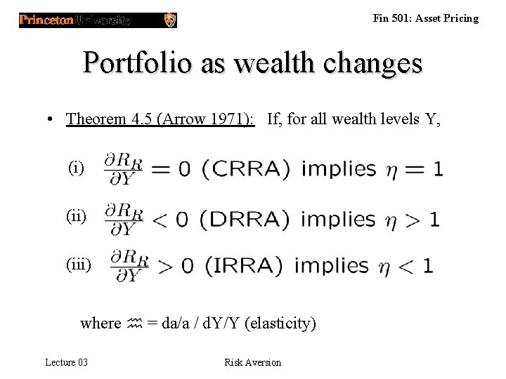
Fin 501: Asset Pricing Portfolio as wealth changes • Theorem 4. 5 (Arrow 1971): If, for all wealth levels Y, (i) (iii) where = da/a / d. Y/Y (elasticity) Lecture 03 Risk Aversion

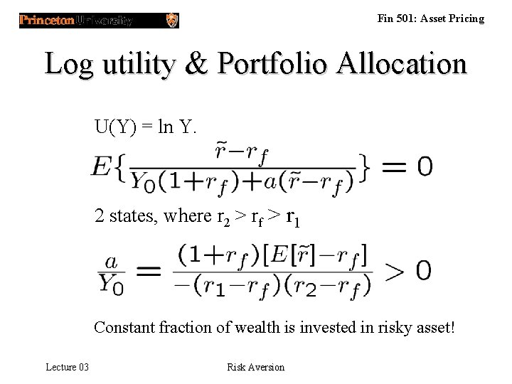
Fin 501: Asset Pricing Log utility & Portfolio Allocation U(Y) = ln Y. 2 states, where r 2 > rf > r 1 Constant fraction of wealth is invested in risky asset! Lecture 03 Risk Aversion

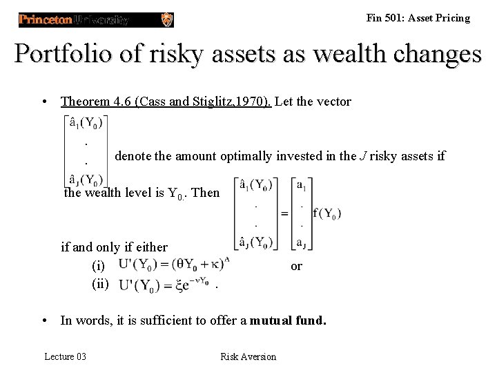
Fin 501: Asset Pricing Portfolio of risky assets as wealth changes • Theorem 4. 6 (Cass and Stiglitz, 1970). Let the vector denote the amount optimally invested in the J risky assets if the wealth level is Y 0. . Then if and only if either (i) (ii) or . • In words, it is sufficient to offer a mutual fund. Lecture 03 Risk Aversion

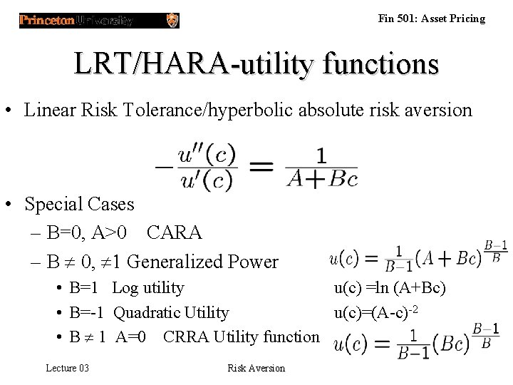
Fin 501: Asset Pricing LRT/HARA-utility functions • Linear Risk Tolerance/hyperbolic absolute risk aversion • Special Cases – B=0, A>0 CARA – B ¹ 0, ¹ 1 Generalized Power • B=1 Log utility u(c) =ln (A+Bc) • B=-1 Quadratic Utility u(c)=(A-c)-2 • B ¹ 1 A=0 CRRA Utility function Lecture 03 Risk Aversion

Fin 501: Asset Pricing Risk Aversion and Savings Behavior • Consumption at t=0 and t=1. (savings decision) • Asset structure – NO risk free bond – One risky asset with random gross return R Lecture 03 Risk Aversion

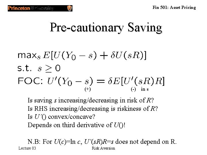
Fin 501: Asset Pricing Pre-cautionary Saving (+) (-) in s Is saving s increasing/decreasing in risk of R? Is RHS increasing/decreasing is riskiness of R? Is U’() convex/concave? Depends on third derivative of U()! N. B: For U(c)=ln c, U’(s. R)R=s does not depend on R. Lecture 03 Risk Aversion

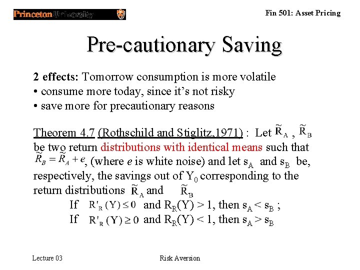
Fin 501: Asset Pricing Pre-cautionary Saving 2 effects: Tomorrow consumption is more volatile • consume more today, since it’s not risky • save more for precautionary reasons Theorem 4. 7 (Rothschild and Stiglitz, 1971) : Let , be two return distributions with identical means such that , (where e is white noise) and let s. A and s. B be, respectively, the savings out of Y 0 corresponding to the return distributions and . If and RR(Y) > 1, then s. A < s. B ; If and RR(Y) < 1, then s. A > s. B Lecture 03 Risk Aversion

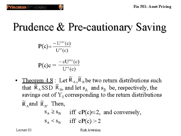
Fin 501: Asset Pricing Prudence & Pre-cautionary Saving P(c)c = • Theorem 4. 8 : Let , be two return distributions such that SSD , and let s. A and s. B be, respectively, the savings out of Y 0 corresponding to the return distributions and . Then, iff c. P(c) 2, and conversely, iff c. P(c) > 2 Lecture 03 Risk Aversion

Fin 501: Asset Pricing Extra material follows! Lecture 03 Risk Aversion

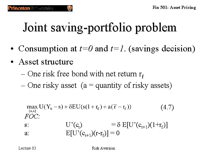
Fin 501: Asset Pricing Joint saving-portfolio problem • Consumption at t=0 and t=1. (savings decision) • Asset structure – One risk free bond with net return rf – One risky asset (a = quantity of risky assets) (4. 7) FOC: s: a: Lecture 03 U’(ct) = d E[U’(ct+1)(1+rf)] E[U’(ct+1)(r-rf)] = 0 Risk Aversion

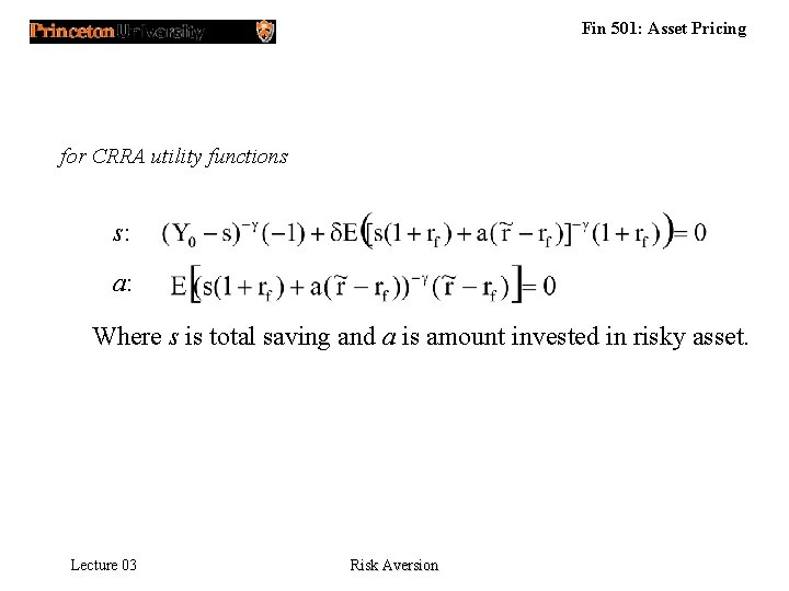
Fin 501: Asset Pricing for CRRA utility functions s: a: Where s is total saving and a is amount invested in risky asset. Lecture 03 Risk Aversion

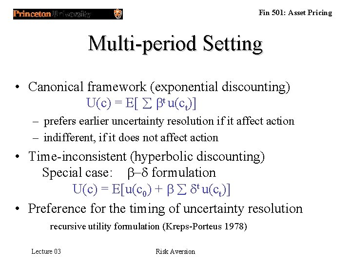
Fin 501: Asset Pricing Multi-period Setting • Canonical framework (exponential discounting) U(c) = E[ å bt u(ct)] – prefers earlier uncertainty resolution if it affect action – indifferent, if it does not affect action • Time-inconsistent (hyperbolic discounting) Special case: b-d formulation U(c) = E[u(c 0) + b å dt u(ct)] • Preference for the timing of uncertainty resolution recursive utility formulation (Kreps-Porteus 1978) Lecture 03 Risk Aversion

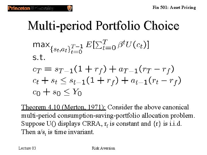
Fin 501: Asset Pricing Multi-period Portfolio Choice Theorem 4. 10 (Merton, 1971): Consider the above canonical multi-period consumption-saving-portfolio allocation problem. Suppose U() displays CRRA, rf is constant and {r} is i. i. d. Then a/st is time invariant. Lecture 03 Risk Aversion

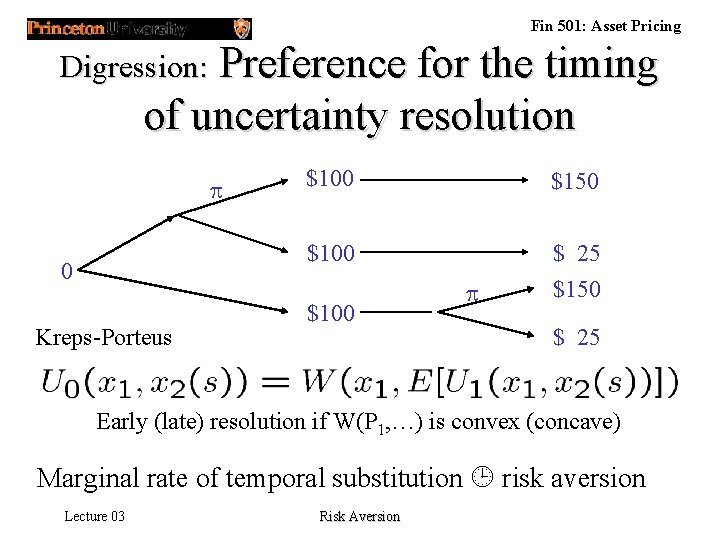
Fin 501: Asset Pricing Digression: Preference for the timing of uncertainty resolution p 0 Kreps-Porteus $100 $150 $100 $ 25 $150 $100 p $ 25 Early (late) resolution if W(P 1, …) is convex (concave) Marginal rate of temporal substitution risk aversion Lecture 03 Risk Aversion