BIOS 501 Lecture 2 Plotting relationships Roderick Little

BIOS 501 Lecture 2 Plotting relationships Roderick Little UNIVERSITY OF MICHIGAN SCHOOL OF PUBLIC HEALTH

Looking at Data-Relationships o o Scatterplots of two variables to visualize relationships Measuring degree of association: Correlation Response vs explanatory variables Fitting a regression line n See IPS Sections 2. 1 -2. 5 2 UNIVERSITY OF MICHIGAN SCHOOL OF PUBLIC HEALTH

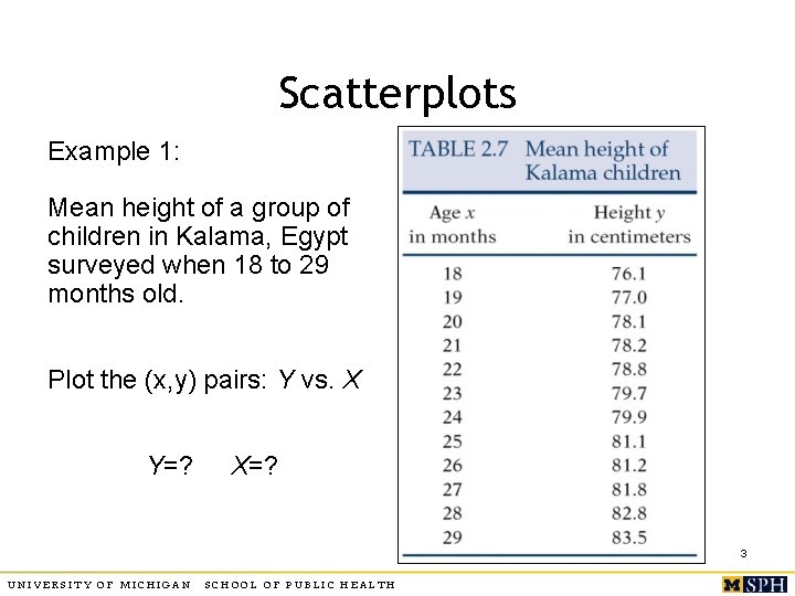
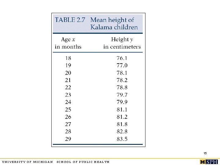
Scatterplots Example 1: Mean height of a group of children in Kalama, Egypt surveyed when 18 to 29 months old. Plot the (x, y) pairs: Y vs. X Y=? X=? 3 UNIVERSITY OF MICHIGAN SCHOOL OF PUBLIC HEALTH

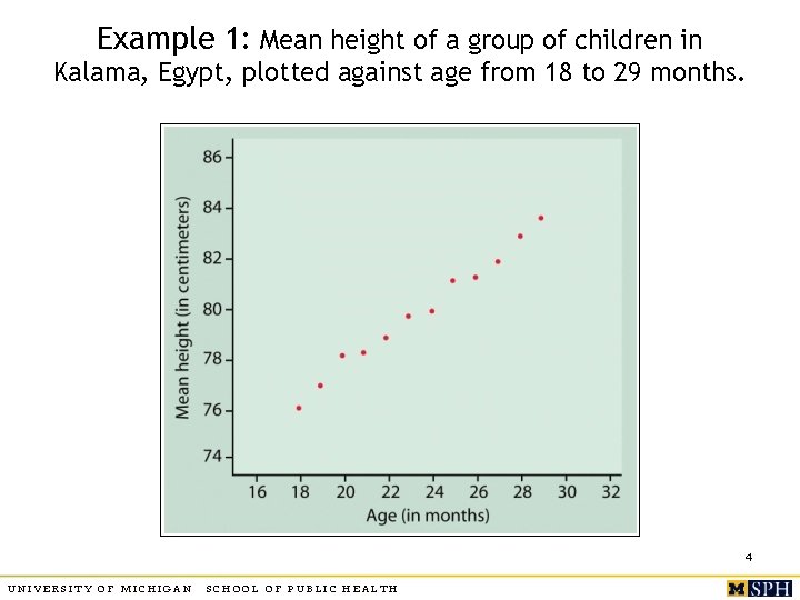
Example 1: Mean height of a group of children in Kalama, Egypt, plotted against age from 18 to 29 months. 4 UNIVERSITY OF MICHIGAN SCHOOL OF PUBLIC HEALTH

Assessing relationships o o Direction: does Y increase with X (positive association), Y decrease with X (negative association)? What is the shape of the underlying form (linear, parabolic, exponential, etc. )? Strength: do the points follow the underlying form quite closely or is there large scatter? Outliers: isolated deviations from overall relationship? 5 UNIVERSITY OF MICHIGAN SCHOOL OF PUBLIC HEALTH

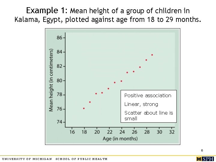
Example 1: Mean height of a group of children in Kalama, Egypt, plotted against age from 18 to 29 months. Positive association Linear, strong Scatter about line is small 6 UNIVERSITY OF MICHIGAN SCHOOL OF PUBLIC HEALTH

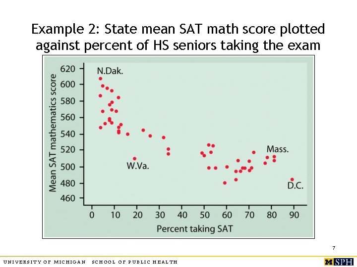
Example 2: State mean SAT math score plotted against percent of HS seniors taking the exam 7 UNIVERSITY OF MICHIGAN SCHOOL OF PUBLIC HEALTH

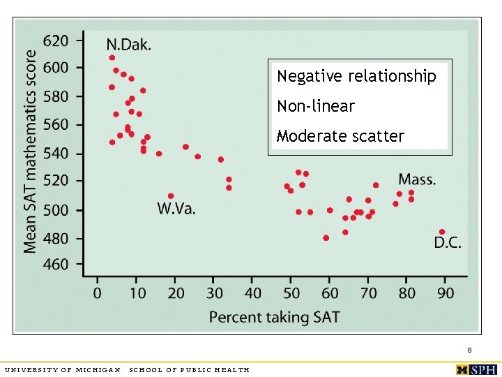
Negative relationship Non-linear Moderate scatter 8 UNIVERSITY OF MICHIGAN SCHOOL OF PUBLIC HEALTH

Association is not causality o o Caution: often spurious, other variables lurking in the background Shorter women have lower risk of heart attack Countries with more TV sets have better life expectancy rates Can’t tell whether a relationship is causal from the plot – depends on other considerations 9 UNIVERSITY OF MICHIGAN SCHOOL OF PUBLIC HEALTH

More on scatter plots o Plotting different categories with different symbols may throw light on data 10 UNIVERSITY OF MICHIGAN SCHOOL OF PUBLIC HEALTH

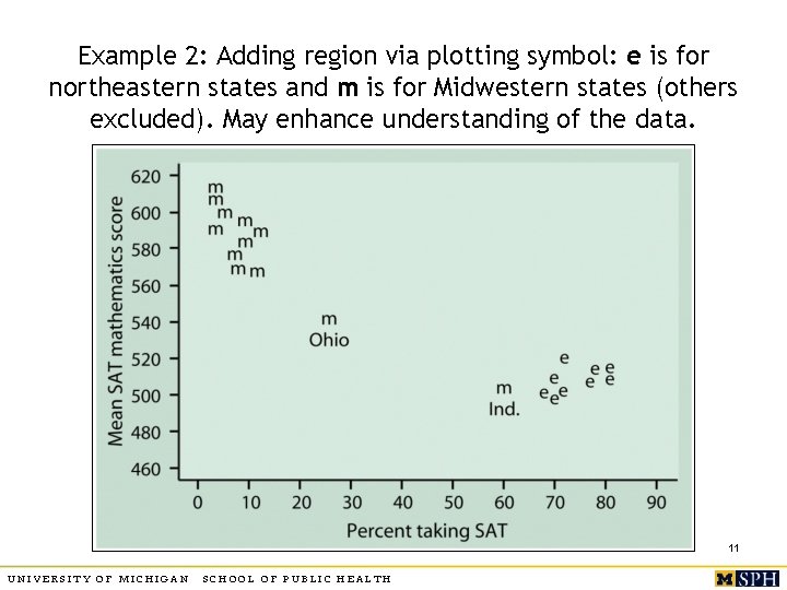
Example 2: Adding region via plotting symbol: e is for northeastern states and m is for Midwestern states (others excluded). May enhance understanding of the data. 11 UNIVERSITY OF MICHIGAN SCHOOL OF PUBLIC HEALTH

More on scatter plots o Plotting on a restricted scale magnifies the relationship, but potential to mislead. 12 UNIVERSITY OF MICHIGAN SCHOOL OF PUBLIC HEALTH

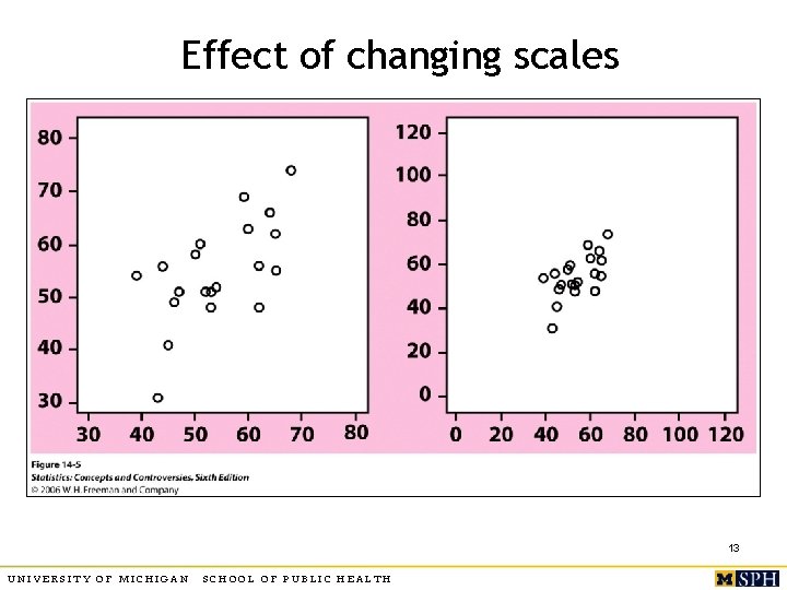
Effect of changing scales 13 UNIVERSITY OF MICHIGAN SCHOOL OF PUBLIC HEALTH

2. 2 Correlation Coefficient o o Linear relationships are quite common. Correlation coefficient r measures strength and direction of a linear relationship between two quantitative variables X and Y. Data structure: (X, Y) pairs measured on n individuals (Weight, blood pressure) or (age, bone-density) measured on a set of subjects 14 UNIVERSITY OF MICHIGAN SCHOOL OF PUBLIC HEALTH

15 UNIVERSITY OF MICHIGAN SCHOOL OF PUBLIC HEALTH

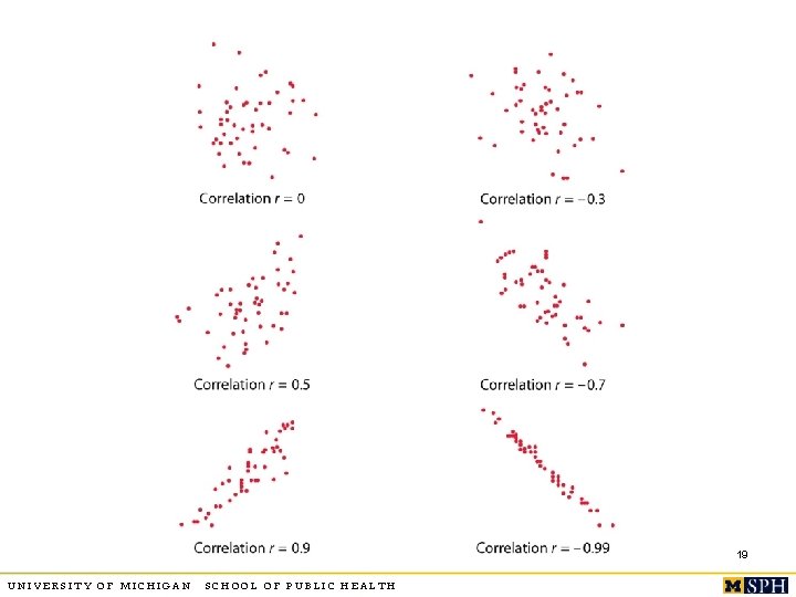
Correlation o o o Lies between -1 and 1 You can switch roles of X and Y, r will remain the same. Unit free, unaffected by linear transformation r positive for positive association, negative for negative association X and Y should both be quantitative. r near 0 implies weak linear relationship, closer to +1 or -1 suggests very strong linear pattern. 16 UNIVERSITY OF MICHIGAN SCHOOL OF PUBLIC HEALTH

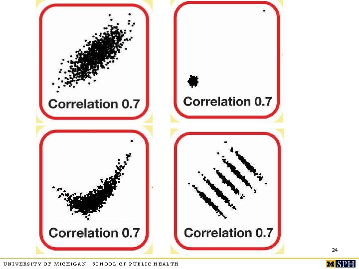
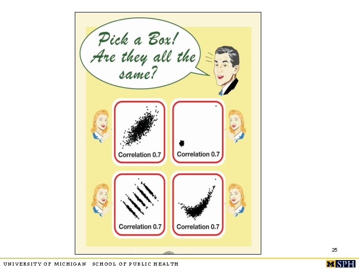
More on correlation o o r is sensitive to outliers. Captures only the strength of “linear” relationship, it could be true that Y and X have a very strong curvilinear relationship but r is close to zero. r = +1 or -1 only when points lie perfectly on a straight line (e. g. Y =2 X+3). In SPSS->Analyze->Correlation->Bivariate 17 UNIVERSITY OF MICHIGAN SCHOOL OF PUBLIC HEALTH

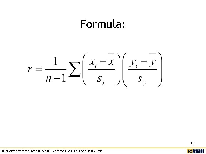
Formula: 18 UNIVERSITY OF MICHIGAN SCHOOL OF PUBLIC HEALTH

19 UNIVERSITY OF MICHIGAN SCHOOL OF PUBLIC HEALTH

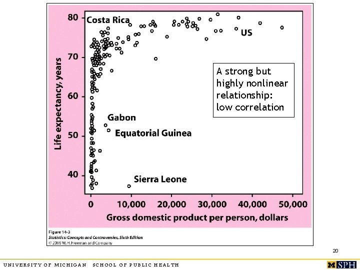
A strong but highly nonlinear relationship: low correlation 20 UNIVERSITY OF MICHIGAN SCHOOL OF PUBLIC HEALTH

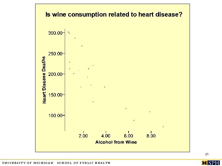
21 UNIVERSITY OF MICHIGAN SCHOOL OF PUBLIC HEALTH

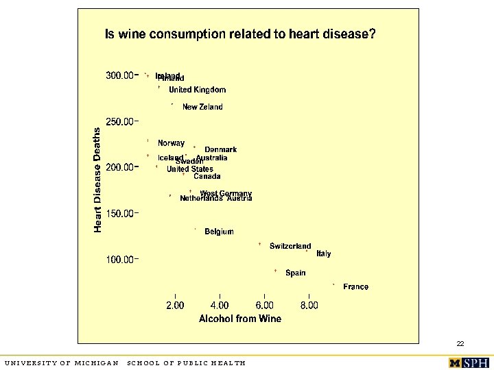
22 UNIVERSITY OF MICHIGAN SCHOOL OF PUBLIC HEALTH

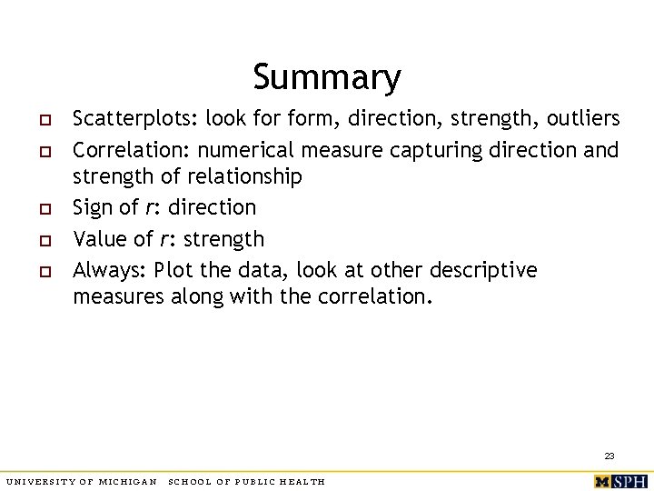
Summary o o o Scatterplots: look form, direction, strength, outliers Correlation: numerical measure capturing direction and strength of relationship Sign of r: direction Value of r: strength Always: Plot the data, look at other descriptive measures along with the correlation. 23 UNIVERSITY OF MICHIGAN SCHOOL OF PUBLIC HEALTH

24 UNIVERSITY OF MICHIGAN SCHOOL OF PUBLIC HEALTH

25 UNIVERSITY OF MICHIGAN SCHOOL OF PUBLIC HEALTH

2. 3 Regression line o Straight line which describes best how the response variable Y changes when the explanatory variable X changes n o Equation of straight lines: n o (We do distinguish between Y and X, cannot switch their roles) y = a+bx (b is the slope, a is the intercept) Task: calculate best a and b for your data. n n Find the line that best fits your data. Use this line to predict y for different values of x. 26 UNIVERSITY OF MICHIGAN SCHOOL OF PUBLIC HEALTH

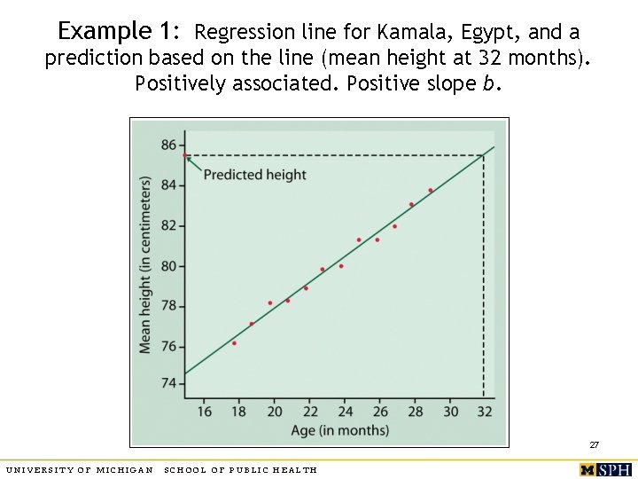
Example 1: Regression line for Kamala, Egypt, and a prediction based on the line (mean height at 32 months). Positively associated. Positive slope b. 27 UNIVERSITY OF MICHIGAN SCHOOL OF PUBLIC HEALTH

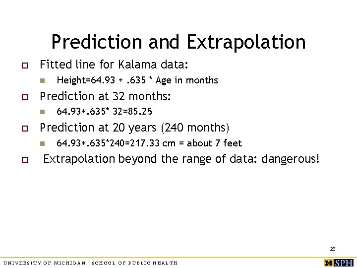
Prediction and Extrapolation o Fitted line for Kalama data: n o Prediction at 32 months: n o 64. 93+. 635* 32=85. 25 Prediction at 20 years (240 months) n o Height=64. 93 +. 635 * Age in months 64. 93+. 635*240=217. 33 cm = about 7 feet Extrapolation beyond the range of data: dangerous! 28 UNIVERSITY OF MICHIGAN SCHOOL OF PUBLIC HEALTH

Least squares regression line o o The line that makes the sum of squares of the vertical distances of the data points from the line as small as possible Observed response = y, predicted response by using the line = yhat Error in prediction: residual = y – yhat Least squares line minimizes sum of squared residuals – see text for detailed formulae. 29 UNIVERSITY OF MICHIGAN SCHOOL OF PUBLIC HEALTH

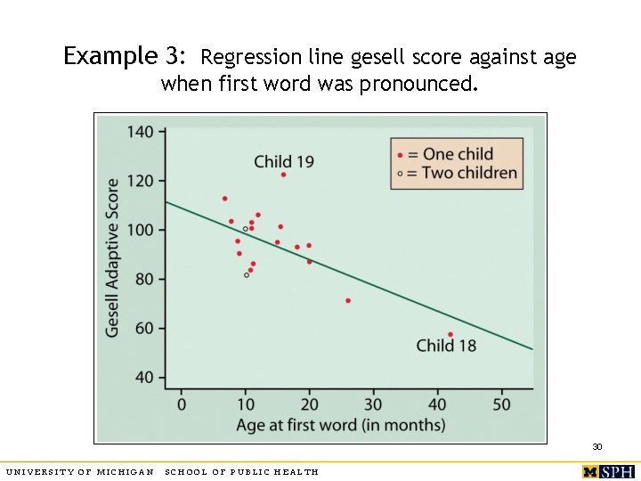
Example 3: Regression line gesell score against age when first word was pronounced. 30 UNIVERSITY OF MICHIGAN SCHOOL OF PUBLIC HEALTH

31 UNIVERSITY OF MICHIGAN SCHOOL OF PUBLIC HEALTH

32 UNIVERSITY OF MICHIGAN SCHOOL OF PUBLIC HEALTH

Properties of regression line o The slope b measures the change in the mean of Y for a one unit increase in X. n n o Slope depends on which variable is X and which is Y. n o E. g. , for Egypt example, height changes an average of. 635 cm for every 1 month increase in age. How about 5 month increase in age? Regression lines of Y on X and X on Y differ. Line passes through the mean of X and mean of Y. 33 UNIVERSITY OF MICHIGAN SCHOOL OF PUBLIC HEALTH

Slope and correlation o o Sign of b is same as the sign of r, indicates the direction of linear association. b is unchanged by adding or subtracting a constant from values of X and Y, but is affected by scale changes in X and Y: n n n E. g. convert: X = age from months to years Slope when X = age in months = 2 (say) Slope when X = age in years= ? 34 UNIVERSITY OF MICHIGAN SCHOOL OF PUBLIC HEALTH

Correlation and Regression o o o The square of correlation, r 2, is the fraction of variation in Y explained by the least squares regression of Y on X. Higher r 2 indicates better fit. r 2=. 989 for Egypt data means 98. 9% of the unexplained variation in height is explained by the fitted regression line with X = age. 35 UNIVERSITY OF MICHIGAN SCHOOL OF PUBLIC HEALTH

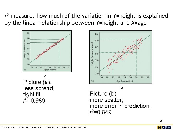
r 2 measures how much of the variation in Y=height is explained by the linear relationship between Y=height and X=age a Picture (a): less spread, tight fit, r 2=0. 989 b Picture (b): more scatter, more error in prediction, r 2=0. 849 36 UNIVERSITY OF MICHIGAN SCHOOL OF PUBLIC HEALTH

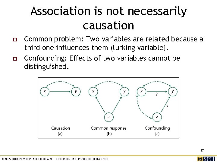
Association is not necessarily causation o o Common problem: Two variables are related because a third one influences them (lurking variable). Confounding: Effects of two variables cannot be distinguished. 37 UNIVERSITY OF MICHIGAN SCHOOL OF PUBLIC HEALTH

Examples o 1. Does birth control reduce fertility in developing countries? n n n o X = use of birth control Y = number of children Expect to see negative association, but in fact association is positive! Confounding variable is number of children at time of birth control – women with many children more likely to use birth control 2. Do higher nursing staff levels reduce “failure to rescue” events in hospitals? n n X = nursing staff level Y = incidence of “failure to rescue” events Confounding variable: Z = severity of illness 38 UNIVERSITY OF MICHIGAN SCHOOL OF PUBLIC HEALTH

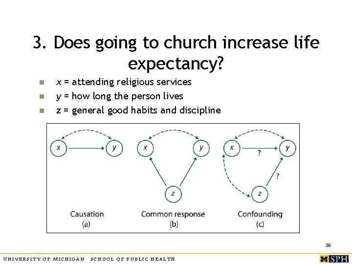
3. Does going to church increase life expectancy? n n n x = attending religious services y = how long the person lives z = general good habits and discipline 39 UNIVERSITY OF MICHIGAN SCHOOL OF PUBLIC HEALTH

4. Does marriage cure poverty? o o “The truth is, the greatest tool to lift children and families from poverty is one that decreases the probability of child poverty by 82%. But it isn’t a government spending program. It’s called marriage. ” U. S. Senator Marco Rubio “It isn’t that having a lasting and successful marriage is a cure for living in poverty… Living in poverty is a barrier to having a lasting and successful marriage. ” Kristi Williams, Ohio State University , quoted in “For Richer, for Poorer” by Annie Lowrey, NYT magazine Feb 9, 2014. 40 UNIVERSITY OF MICHIGAN SCHOOL OF PUBLIC HEALTH

Summary o o Use scatterplots, correlation and regression to capture association between two quantitative variables. Distinguish between association and causation. n o There could be more than one explanation of association. More on regression later. 41 UNIVERSITY OF MICHIGAN SCHOOL OF PUBLIC HEALTH