Extremes in a Varied Climate Chris Ferro Climate

Extremes in a Varied Climate Chris Ferro Climate Analysis Group Department of Meteorology University of Reading 1. Significance of distributional changes 2. Extreme-value analysis of gridded data

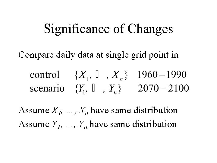
Significance of Changes Compare daily data at single grid point in Assume X 1, …, Xn have same distribution Assume Y 1, …, Yn have same distribution

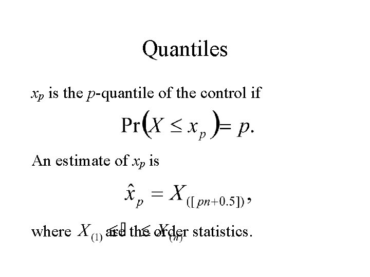
Quantiles xp is the p-quantile of the control if An estimate of xp is where are the order statistics.

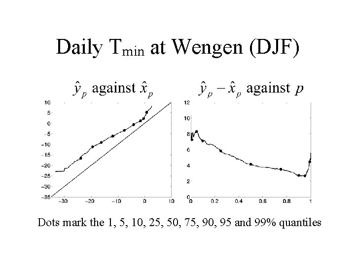
Daily Tmin at Wengen (DJF) Dots mark the 1, 5, 10, 25, 50, 75, 90, 95 and 99% quantiles

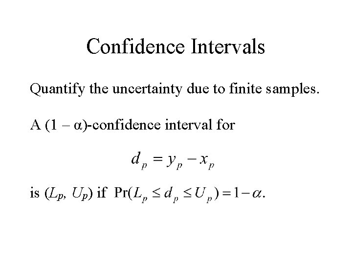
Confidence Intervals Quantify the uncertainty due to finite samples. A (1 – α)-confidence interval for is (Lp, Up) if

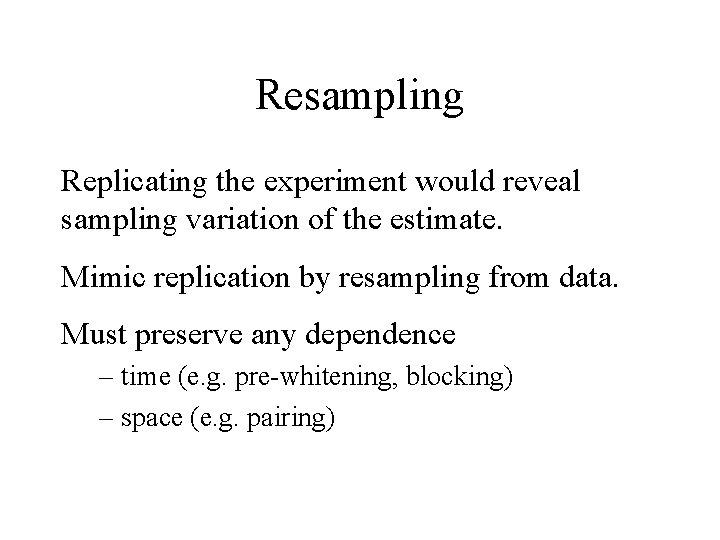
Resampling Replicating the experiment would reveal sampling variation of the estimate. Mimic replication by resampling from data. Must preserve any dependence – time (e. g. pre-whitening, blocking) – space (e. g. pairing)

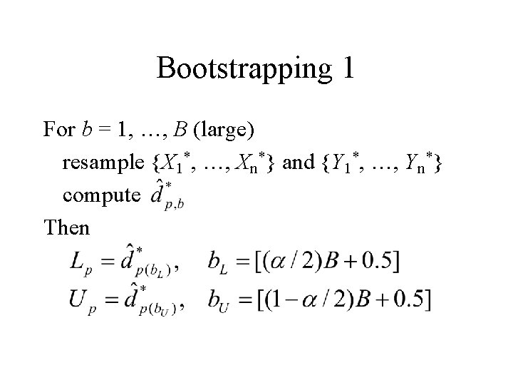
Bootstrapping 1 For b = 1, …, B (large) resample {X 1*, …, Xn*} and {Y 1*, …, Yn*} compute Then

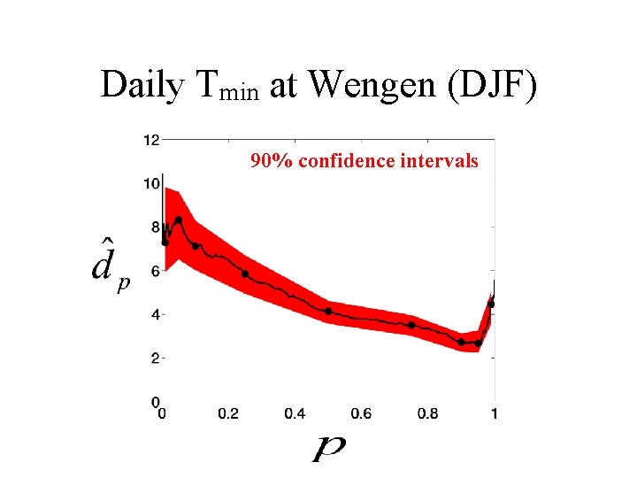
Daily Tmin at Wengen (DJF) 90% confidence intervals

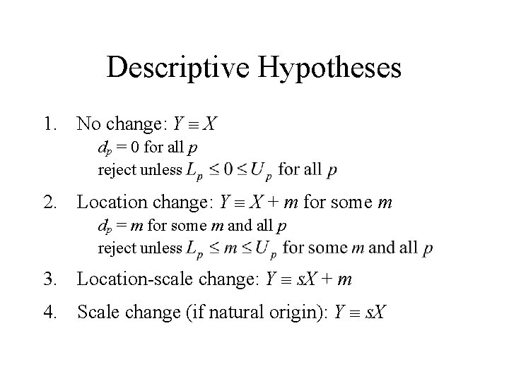
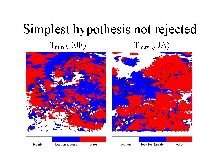
Descriptive Hypotheses 1. No change: Y X dp = 0 for all p reject unless 2. Location change: Y X + m for some m dp = m for some m and all p reject unless 3. Location-scale change: Y s. X + m 4. Scale change (if natural origin): Y s. X

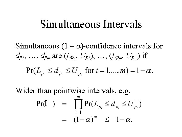
Simultaneous Intervals Simultaneous (1 – α)-confidence intervals for dp 1, …, dpm are (Lp 1, Up 1), …, (Lpm, Upm) if Wider than pointwise intervals, e. g.

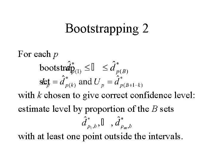
Bootstrapping 2 For each p bootstrap set with k chosen to give correct confidence level: estimate level by proportion of the B sets with at least one point outside the intervals.

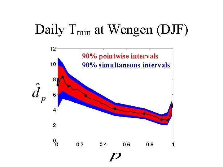
Daily Tmin at Wengen (DJF) 90% pointwise intervals 90% simultaneous intervals

Simplest hypothesis not rejected Tmin (DJF) Tmax (JJA)

Other issues • Interpretation tricky when distributions change within samples: adjust for trends • Bootstrapping quantiles is difficult: more sophisticated bootstrap methods • Field significance • Computational cost

Conclusions • Quantiles describe entire distribution • Confidence intervals quantify uncertainty • Bootstrapping can account for dependence

Extreme-value Analysis • Summarise extremes at each grid point • Estimate return levels and other quantities • Framework for quantifying uncertainty • Summarise model output • Validate and compare models • Downscale model output

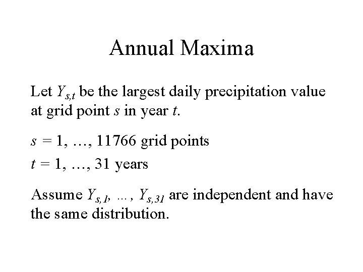
Annual Maxima Let Ys, t be the largest daily precipitation value at grid point s in year t. s = 1, …, 11766 grid points t = 1, …, 31 years Assume Ys, 1, …, Ys, 31 are independent and have the same distribution.

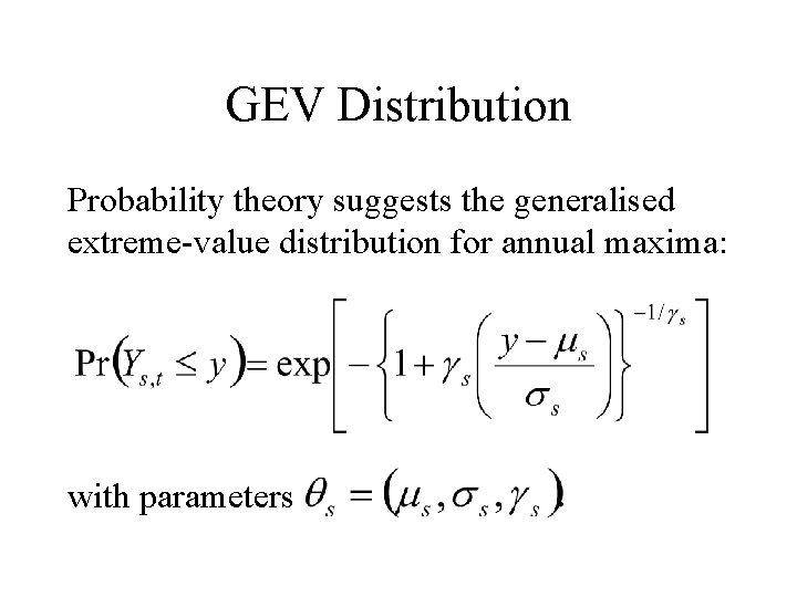
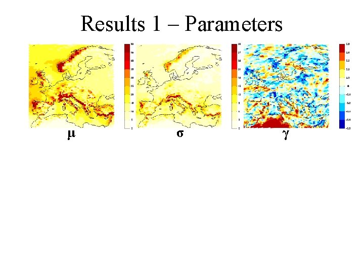
GEV Distribution Probability theory suggests the generalised extreme-value distribution for annual maxima: with parameters

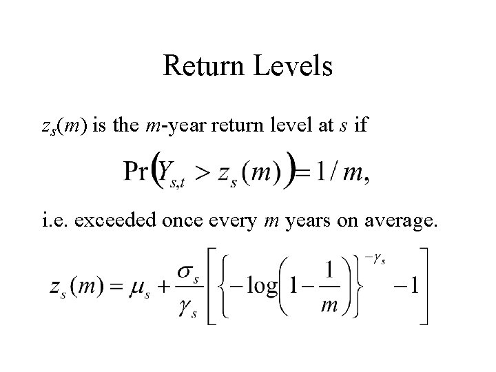
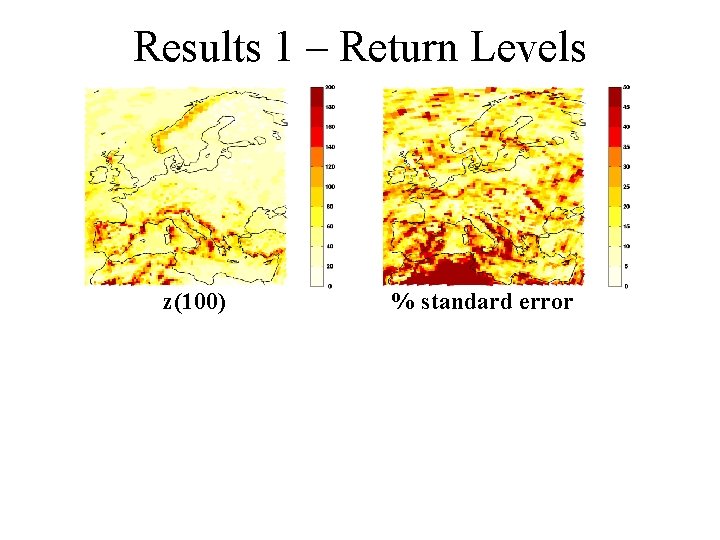
Return Levels zs(m) is the m-year return level at s if i. e. exceeded once every m years on average.

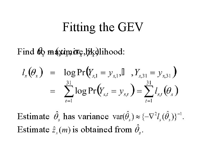
Fitting the GEV Find to maximise likelihood: Estimate has variance is obtained from

Results 1 – Parameters μ σ γ

Results 1 – Return Levels z(100) % standard error

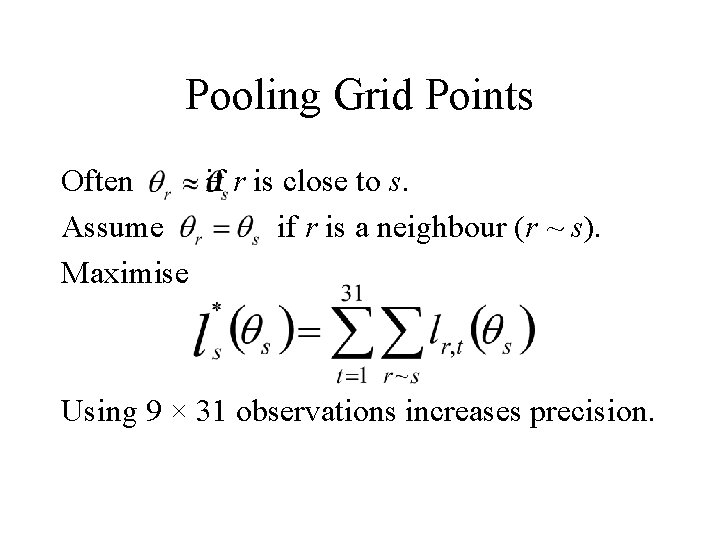
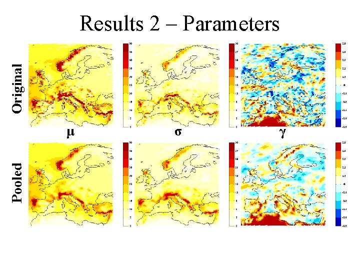
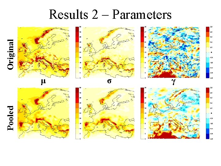
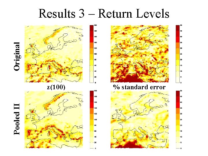
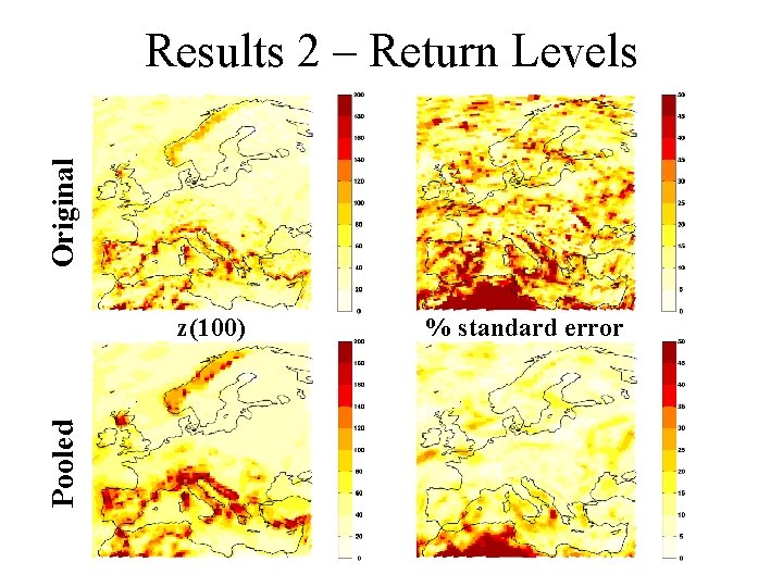
Pooling Grid Points Often if r is close to s. Assume if r is a neighbour (r ~ s). Maximise Using 9 × 31 observations increases precision.

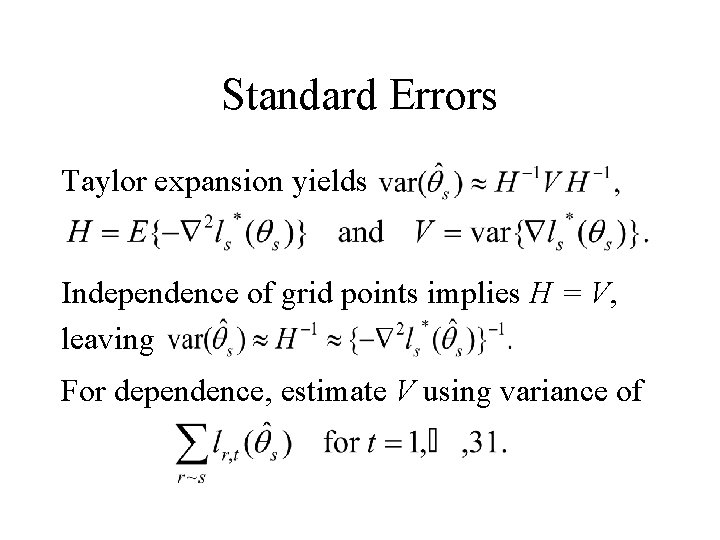
Standard Errors Taylor expansion yields Independence of grid points implies H = V, leaving For dependence, estimate V using variance of

Original Results 2 – Parameters Pooled μ σ γ

Original Results 2 – Return Levels Pooled z(100) % standard error

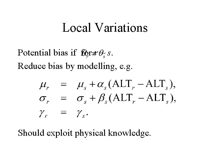
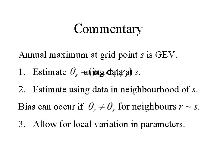
Local Variations Potential bias if for r ~ s. Reduce bias by modelling, e. g. Should exploit physical knowledge.

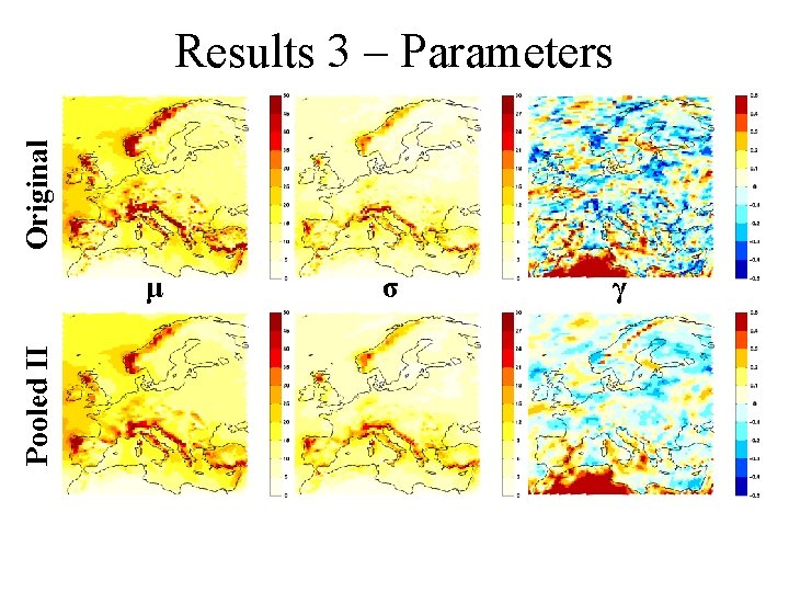
Original Results 3 – Parameters Pooled II μ σ γ

Original Results 2 – Parameters Pooled μ σ γ

Original Results 3 – Return Levels Pooled II z(100) % standard error

Original Results 2 – Return Levels Pooled z(100) % standard error

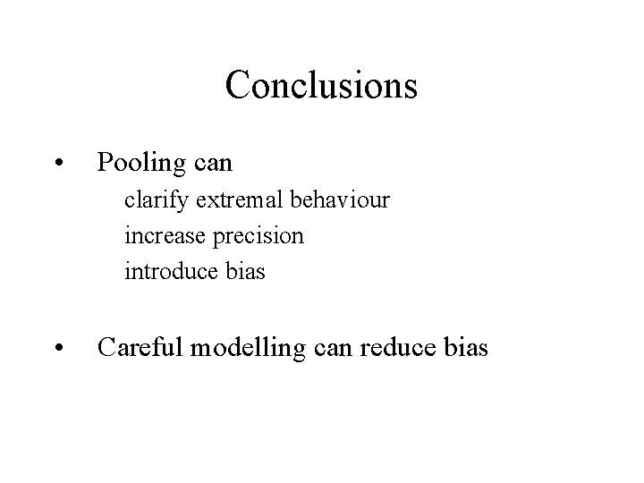
Conclusions • Pooling can clarify extremal behaviour increase precision introduce bias • Careful modelling can reduce bias

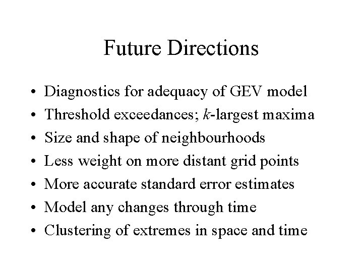
Future Directions • • Diagnostics for adequacy of GEV model Threshold exceedances; k-largest maxima Size and shape of neighbourhoods Less weight on more distant grid points More accurate standard error estimates Model any changes through time Clustering of extremes in space and time

References • Davison & Hinkley (1997) Bootstrap Methods and their Application. Cambridge University Press. • Davison & Ramesh (2000) Local likelihood smoothing of sample extremes. J. Royal Statistical Soc. B, 62, 191– 208. • Smith (1990) Regional estimation from spatially dependent data. www. unc. edu/depts/statistics/faculty/rsmith. html • Wilks (1997) Resampling hypothesis tests for autocorrelated fields. J. Climate, 10, 65 – 82. c. a. t. ferro@reading. ac. uk www. met. rdg. ac. uk/~sws 02 caf

Commentary Annual maximum at grid point s is GEV. 1. Estimate using data at s. 2. Estimate using data in neighbourhood of s. Bias can occur if 3. Allow for local variation in parameters.