Excel 2007 Microsoft Office Excel 2007 Formulas Functions

Excel 2007 Microsoft Office Excel 2007 Formulas, Functions, Formatting, and Web Queries

Formulas, Functions, Formatting, and Web Queries Objectives Chapter Topics End of Chapter Exercises Assignments

Objectives • • You will have mastered the material in this chapter when you can: Enter formulas using the • Set margins, headers, and keyboard and Point mode footers in Page Layout Apply the AVERAGE, MAX, View and MIN functions • Preview and print versions Verify a formula using of a worksheet Range Finder • Use a Web query to get Apply a theme to a real-time data from a workbook Web site Add conditional • Rename sheets in a formatting to cells workbook Change column width and • E-mail the active row height workbook from within Check the spelling of a Excel worksheet (Continued on Next Page) Main Menu Back Next

Formulas, Functions, Formatting, And Web Queries Introduction See Page EX 82 in Your Textbook • Using formulas and functions to create a worksheet • A function is a prewritten formula that is built into Excel • Other new topics include: • smart tags and option buttons • verifying formulas • applying a theme to a worksheet • adding borders • formatting numbers and text • using conditional formatting • changing the widths of columns and heights of rows • spell checking, e-mailing from within an application, Main Menu Back Next

Project – Worksheet with Formulas, Functions, And Web Queries The project in the chapter follows proper design guidelines and uses Excel to create the two worksheets shown in Figure 2 -1 DUE next Tuesday 3/16 Figure 2 -1(a) Figure 2 -1(b) Back Next

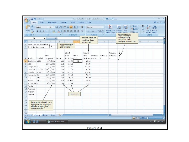
Overview You will be: • Entering formulas an applying functions. • Adding conditional formatting. • Applying a theme. • Working with the Page Layout View. • Printing a part of a worksheet. • Performing a Web query. • E-mailing the worksheet. Figure 2 -3

To do: Start Excel 1. 2. 3. 4. 5. 6. Click the Start Button. Point to All Programs to display the All Programs list. Click Microsoft Office in the All Programs list. Click Microsoft Office Excel to start Excel. Maximize the Excel window if necessary. Maximize the Excel worksheet if necessary.

To do: To Enter the Worksheet Title and Subtitle Entering titles and numbers into a worksheet would be done by: Step 1: If necessary, select cell A 1. Type “Silver Dollars Stock Club” in the cell and then press the Down Arrow key to enter the worksheet title in cell A 1. Step 2: Type “Portfolio Summary” in cell A 2 and the press the Down Arrow key to enter the worksheet subtitle in cell A 2. Main Menu

To do: Enter the Portfolio Summary Data Enter the column headers Enter the data

To do: Enter the Row Titles Step 1: Select cell A 13. type “Totals” and then press the Down Arrow key. Type “Average” in cell A 14 and then press the Down Arrow key. Step 2: Type “Highest” in cell A 15 and then press the Down Arrow key. Type “Lowest” in cell A 16 and then press the ENTER key. Select cell F 4.

To Change Workbook Properties and Save the Workbook You should change the workbook properties the first time you save the workbook.

Entering Formulas One of the reasons Excel is such a valuable tool is that you can assign a formula to a cell and Excel will calculate the results. Note: Your textbook has more information on the topic.

To Enter a Formula Using the Keyboard

EX 92 Arithmetic Operations See Page EX 92 in Your Textbook Note: Your textbook has more information on the topic. Main Menu Back Next

EX 92 Order of Operations See Page EX 92 in Your Textbook Note: Your textbook has more information on the topic. Main Menu Back Next

To Enter Formulas Using Point Mode Point mode allows you to select cells for use in a formula by using the mouse.

To Copy Formulas Using the Fill Handle

Smart Tags and Option Buttons Excel can identify certain action to take on specific data in workbooks using smart tags. Data labeled with smart tags includes dates, financial symbols, people’s names and more. To use smart tags, you must turn on smart tags using the Auto. Correct Options in the Excel Options dialog box. To change Auto. Correct options, click the Office Button. , click the Excel Options button on the Office Button menu, click Proofing and then click Auto. Correct Options. Once smart tags are turned on, Excel places a small purple triangle , called a smart tag indicator, in a cell to indicate that a smart tag is available. Note: Your textbook has more information on the topic. Main Menu Back Next

To do: Determine Totals Using the Sum Button To determine the Sum (For the Textbook Project) Step 1: Select cell F 13. Click the Sum button on the Ribbon and then click the ENTER button. Step 2: Select the range H 13: I 13. Click the Sum button on the Ribbon to display the totals in row 13 as shown in Figure 2 -14

To do: Determine Total Percent Gain/Loss In the textbook project you would: Step 1: Select cell J 12 and then point to the fill handle. Step 2: Drag the fill handle down through cell J 13 to copy the formula in cell J 12 to cell J 13. NOTE: A blank cell in Excel has a numerical value of zero.

Using the AVERAGE, MAX, and MIN Functions Excel includes prewritten formulas called functions to help you compute some statistics. A function takes a value or values, performs an operation, and returns a result to the cell. The values that you use with a function are called arguments. All functions begin with an equal sign and include the arguments in parentheses after the function name.

To Determine the Average of a Range of Numbers Using the Keyboard and Mouse The AVERAGE function sums the numbers in the specified range and then divides the sum by the number of nonzero cells in the range.

To do: Determine the Highest Number in a Range of Numbers Using the Insert Function Box The MAX function displays the highest value in a range.

To do: Determine the Lowest Number in a Range of Numbers Using the Sum Menu The MIN function determines the lowest (minimum) number in a range.

To do: Copy a Range of Cells across Columns to an Adjacent Range Using the Fill Handle

To do: Formatting the workbook • Change theme • Format the worksheet titles • Change the Background Color • Apply a Box Border to the Worksheet Title and Subtitle • Center data • Format dates • Formatting numbers using the ribbon • Apply a percent style • Fix number of decimal places

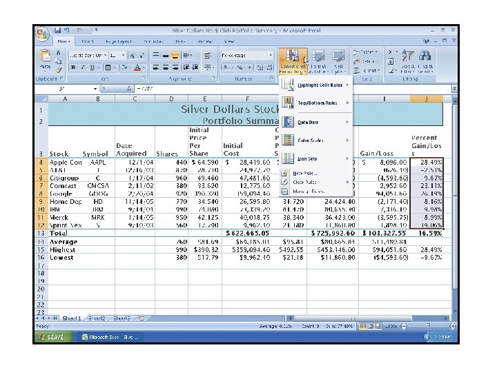
Conditional Formatting Excel lets you apply formatting that appears only when the value in a cell meets conditions that you specify. This type of formatting is called conditional formatting. A condition, which is made up of two values and a relational operator, is true or false for each cell in the range.

To do: Apply Conditional Formatting (Part 1) See Page EX 119 in Your Textbook For your textbook project you would: Step 1: Select the range J 4: J 12. Click the Conditional Formatting button on the Ribbon to display the Conditional Formatting gallery. Step 2: Click New Rule in the Conditional Formatting gallery to display the New Formatting Rule dialog box. – Click “Format only cells that contain” in the Select a Rule Type area. – In the Edit Rule Description area, click the box arrow in the relational operator box and then select less than. – Type : O” (zero) in the rightmost box in the Edit the Rule Description area. Figure 2 -48 Figure 2 -49

To do: Apply Conditional Formatting (Part 2) For your textbook project you would: Step 3: Click the Format button. When Excel displays the Format Cells dialog box, click the fill tab and then click the light red color in column 7, row 2. Figure 2 -50

To do: Apply Conditional Formatting (Part 3) For your textbook project you would: Step 4: Click the OK button to close the Format Cells dialog box and display the New Formatting Rule dialog box with the desired color displayed in the Preview box. Figure 2 -51

To do: Apply Conditional Formatting (Part 3) For your textbook project you would: Step 5: Click the OK button to assign the conditional format to the range J 4: J 12. Figure 2 -52

Conditional Formatting Operators See Page EX 121. You can specify a New Formatting Rule and in the process select a relational operator. The eight different relational operators from which you can choose for conditional formatting in the New Formatting Rule dialog box are summarized in Table 2 -5.

Changing the Widths of Columns and Heights of Rows When Excel starts and displays a blank worksheet on the screen, all of the columns have a default width of 8. 43 characters, or 64 pixels. A character is defined as a letter, number, symbol, or punctuation mark in 11 -point Calibri font, the default font used by Excel. An average of 8. 43 characters in 11 point Calibri font will fit in a cell. Another measure of height and width of cells is pixels, which is short for picture element. A pixel is a dot on the screen that contains a color. The size of the dot is based on your screen’s resolution. At a common resolution of 1024 X 768, 1024 pixels appear across the screen and 768 pixels appear down the screen for a total of 786, 432 pixels. It is these 786, 432 pixels that form the font and other items you see on the screen.

Checking Spelling Excel has a spell checker you can use to check the worksheet for spelling errors. The spell checker looks for spelling errors by comparing words on the worksheet against words contained in its standard dictionary. If you often use specialized terms that are not in the standard dictionary, you may want to add them to a custom dictionary using the Spelling dialog box. When the spell checker finds a word that is not in either dictionary, it displays the word in the Spelling dialog box. You then can correct it if it is misspelled.

To do: Check Spelling on the Worksheet (Part 1) Step 1: Click cell A 3 and then type “Stcok” to misspell the word “Stock”. Click cell A 1. Click the Review tab on the Ribbon. Click the Spelling button on the Ribbon to run the spell checker and display the misspelled word, “Stcok”, in the Spelling dialog box. Figure 2 -61

To do: Check Spelling on the Worksheet (Part 2) Step 2: With the word “Stock” highlighted in the Suggestions list, click the Change button to change the misspelled word, “Stcok”, to the correct word, “Stock”. Figure 2 -62

Preparing to Print the Worksheet Excel allows for a great deal of customization in how a worksheet appears when printed. For example, the margins on the page can be adjusted. A header or footer can be added to each printed page as well. Excel also has the capability to work on the worksheet in Page Layout View allows you to create or modify a worksheet while viewing how it will look in printed format. The default view that you have worked in up until this point in the book is called Normal View.

To do: Change the Worksheet’s Margins, Header, and Orientation in Page Layout View (Part 1) Step 1: Click the Page Layout view button on the status bar to view the worksheet in Page Layout.

To Change the Worksheet’s Margins, Header, and Orientation in Page Layout View (Part 2) Step 2: Click the Page Layout tab on the Ribbon. Click the Margins button on the Ribbon to display the Margins gallery.

Previewing and Printing the Worksheet By previewing the worksheet, however, you see exactly how it will look without generating a printout. Previewing a worksheet using the Print Preview command can save time, paper, and the frustration of waiting for a printout only to discover it is not what you want. • Preview and print a worksheet • Print a section of a worksheet Next

Displaying and Printing the Formulas Version of the Worksheet Thus far, you have been working with the values version of the worksheet, which shows the results of the formulas you have entered, rather than the actual formulas. Excel also can display and print the formulas version of the worksheet, which shows the actual formulas you have entered rather than the resulting values. You can toggle between the values version and formulas version by holding down the CTRL key while pressing the ACCENT MARK (`) key, which is located to the left of the number 1 key on the keyboard. The formulas version is useful for debugging a worksheet. Debugging is the process of finding and correcting errors in the worksheet.

To do: Display the Formulas in the Worksheet and Fit the Printout on One Page Step 1: Press CTRL + ACCENT MARK (`). Excel displays the formulas version of the worksheet – click the right horizontal scroll arrow until column J appears to display the worksheet with formulas. Step 2: If necessary, click the Page Layout tab on the Ribbon and then click the Page Setup Dialog Box Launcher to display the Page Setup dialog box. Step 3: Click the Print button in the Page Setup dialog box to print the formulas in the worksheet on one page in landscape orientation. When Excel displays the Print dialog box, click the OK button.

To do: Display the Formulas in the Worksheet and Fit the Printout on One Page Step 4: After viewing and printing the formulas version, press CTRL + ACCENT MARK (`) to instruct Excel to display the values version. Click the left horizontal scroll arrow until column A appears.

Importing External Data from a Web Source Using a Web Query You can import data stored on a Web site using a Web query.

To do: Import Data from a Web Source Using a Web Query Although you can have a Web query return data to a blank workbook, the steps in your textbook describes how to import data returned by a stock related Web query.

Chapter Summary You learned many things in the development of the textbook project: how to enter formulas, calculate an average, find the highest and lowest numbers in a range, verify formulas using Range Finder, draw borders, align text, format numbers, change column widths and row heights, and add conditional formatting to a range of numbers. In addition, you learned to spell check a worksheet, preview a worksheet, print a section of a worksheet, display and print the formulas version of the worksheet using the Fit to piton, complete a Web query, rename sheet tabs, and send an e-mail directly from within Excel with the opened workbook as an attachment.

In The Lab Create a workbook using the guidelines, concepts, and skills presented in the chapter. Labs are listed in order of increasing difficulty. In the Lab See Page EX 149 -155 Lab 1: Sales Analysis Worksheet Lab 2: Balance Due Worksheet Lab 3: Equity Web Queries NOTE: See your textbook for complete information on the labs listed above.