Excel Solver IE 469 Spring 2017 Excels Solver


- Slides: 20

Excel Solver IE 469 Spring 2017

Excel’s Solver • Use Excel’s Solver as a tool to assist the decision maker in identifying the optimal solution for a business decision. • Business decisions are often subject to constraints or business rules to solve business problems. • Solver can be used for decisions, such as, maximizing profit or reducing costs. Slide 2

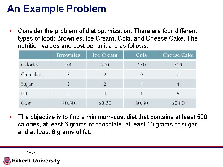
An Example Problem • Consider the problem of diet optimization. There are four different types of food: Brownies, Ice Cream, Cola, and Cheese Cake. The nutrition values and cost per unit are as follows: • The objective is to find a minimum-cost diet that contains at least 500 calories, at least 6 grams of chocolate, at least 10 grams of sugar, and at least 8 grams of fat. Slide 3

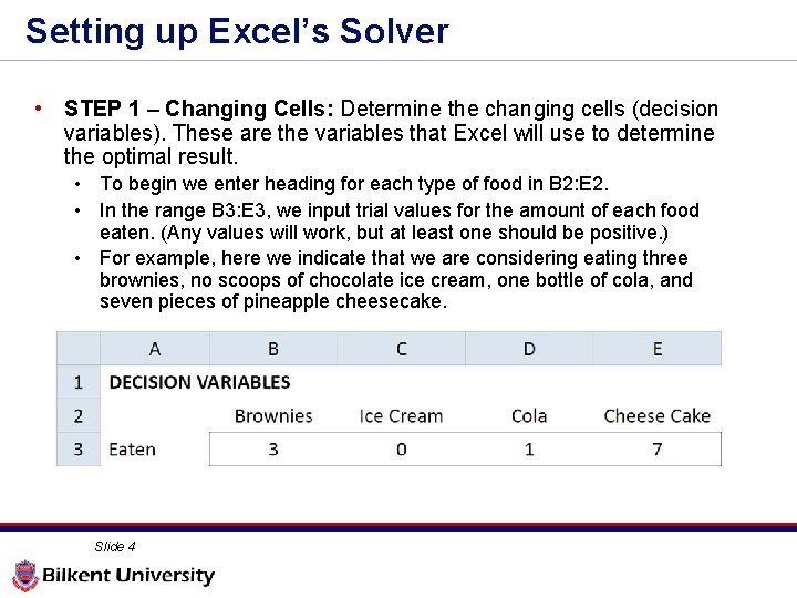
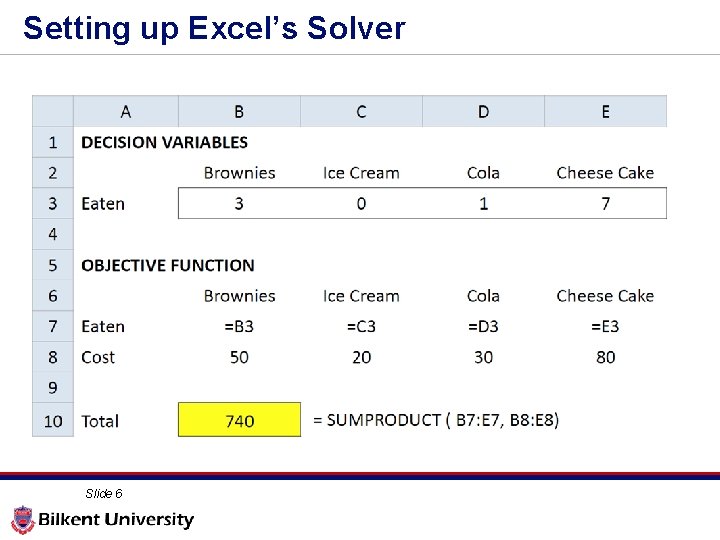
Setting up Excel’s Solver • STEP 1 – Changing Cells: Determine the changing cells (decision variables). These are the variables that Excel will use to determine the optimal result. • To begin we enter heading for each type of food in B 2: E 2. • In the range B 3: E 3, we input trial values for the amount of each food eaten. (Any values will work, but at least one should be positive. ) • For example, here we indicate that we are considering eating three brownies, no scoops of chocolate ice cream, one bottle of cola, and seven pieces of pineapple cheesecake. Slide 4

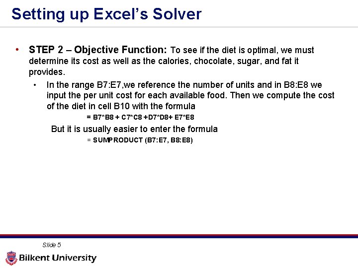
Setting up Excel’s Solver • STEP 2 – Objective Function: To see if the diet is optimal, we must determine its cost as well as the calories, chocolate, sugar, and fat it provides. • In the range B 7: E 7, we reference the number of units and in B 8: E 8 we input the per unit cost for each available food. Then we compute the cost of the diet in cell B 10 with the formula = B 7*B 8 + C 7*C 8 +D 7*D 8+ E 7*E 8 But it is usually easier to enter the formula = SUMPRODUCT (B 7: E 7, B 8: E 8) Slide 5

Setting up Excel’s Solver Slide 6

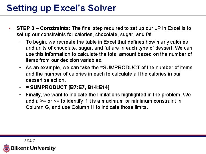
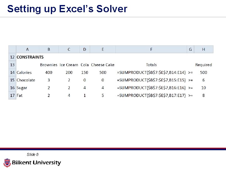
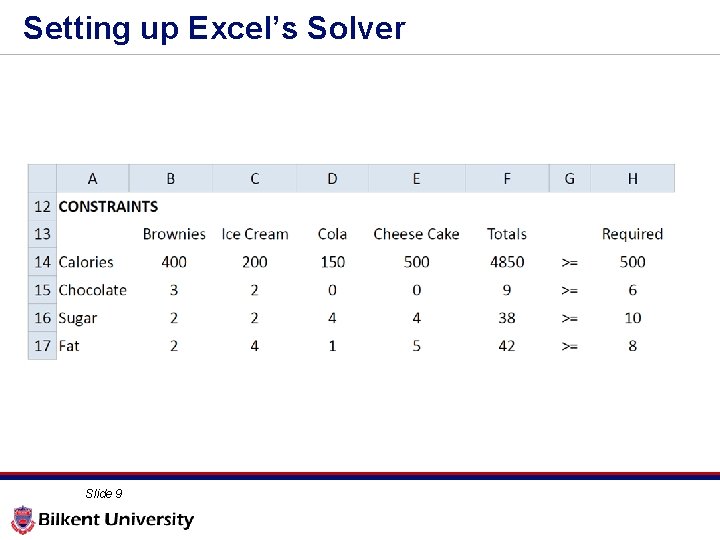
Setting up Excel’s Solver • STEP 3 – Constraints: The final step required to set up our LP in Excel is to set up our constraints for calories, chocolate, sugar, and fat. • To begin, we recreate the table in Excel that defines how many calories and units of chocolate, sugar, and fat are in each type of dessert. We can use this information to calculate the total amount based on the number of items from our decision variables. • As an example, we can take the =SUMPRODUCT of the number of items and the number of calories in each to calculate all the calories in our dessert selection. • = SUMPRODUCT (B 7: E 7, B 14: E 14) • Finally, we want to indicate the limitations highlighted in the problem. We add a >= or <= to identify if it is a maximum or minimum constraint in Column G, and use Column H to indicate those limits. Slide 7

Setting up Excel’s Solver Slide 8

Setting up Excel’s Solver Slide 9

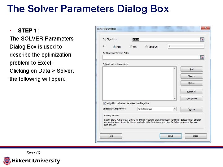
The Solver Parameters Dialog Box • STEP 1: The SOLVER Parameters Dialog Box is used to describe the optimization problem to Excel. Clicking on Data > Solver, the following will open: Slide 10

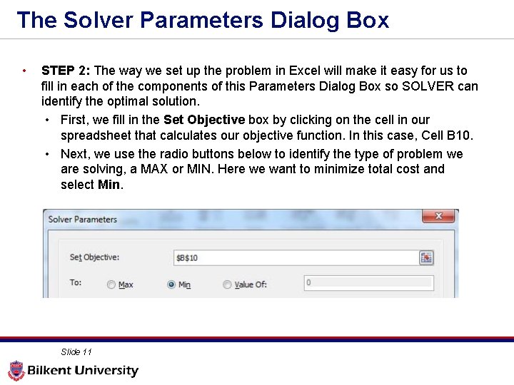
The Solver Parameters Dialog Box • STEP 2: The way we set up the problem in Excel will make it easy for us to fill in each of the components of this Parameters Dialog Box so SOLVER can identify the optimal solution. • First, we fill in the Set Objective box by clicking on the cell in our spreadsheet that calculates our objective function. In this case, Cell B 10. • Next, we use the radio buttons below to identify the type of problem we are solving, a MAX or MIN. Here we want to minimize total cost and select Min. Slide 11

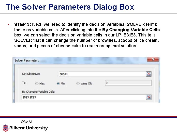
The Solver Parameters Dialog Box • STEP 3: Next, we need to identify the decision variables. SOLVER terms these as variable cells. After clicking into the By Changing Variable Cells box, we can select the decision variable cells in our LP, B 3: E 3. This tells SOLVER that it can change the number of brownies, scoops of ice cream, sodas, and pieces of cheese cake to reach an optimal solution. Slide 12

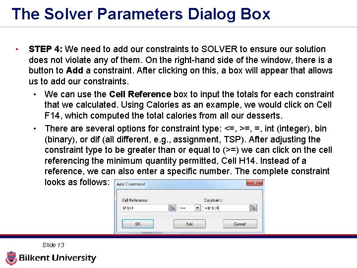
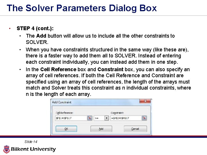
The Solver Parameters Dialog Box • STEP 4: We need to add our constraints to SOLVER to ensure our solution does not violate any of them. On the right-hand side of the window, there is a button to Add a constraint. After clicking on this, a box will appear that allows us to add our constraints. • We can use the Cell Reference box to input the totals for each constraint that we calculated. Using Calories as an example, we would click on Cell F 14, which computed the total calories from all our desserts. • There are several options for constraint type: <=, >=, =, int (integer), bin (binary), or dif (all different, e. g. , assignment, TSP). After adjusting the constraint type to be greater than or equal to (>=) we can click on the cell referencing the minimum quantity permitted, Cell H 14. Instead of a reference, we can also enter a specific number. The complete constraint looks as follows: Slide 13

The Solver Parameters Dialog Box • STEP 4 (cont. ): • The Add button will allow us to include all the other constraints to SOLVER. • When you have constraints structured in the same way (like these are), there is a faster way to add them all to SOLVER. Instead of entering each constraint individually, you can instead add them in one step. • In the Cell Reference box and Constraint box, you can also specify an array of cell references. If both the Cell Reference and Constraint are specified using an array of cell references, the length of the arrays must match and Solver treats this constraint as n individual constraints, where n is the length of each array. Slide 14

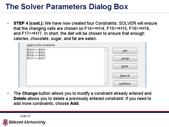
The Solver Parameters Dialog Box • STEP 4 (cont. ): We have now created four Constraints. SOLVER will ensure that the changing cells are chosen so F 14>=H 14, F 15>=H 15, F 16>=H 16, and F 17>=H 17. In short, the diet will be chosen to ensure that enough calories, chocolate, sugar, and fat are eaten. • The Change button allows you to modify a constraint already entered and Delete allows you to delete a previously entered constraint. If you need to add more constraints, choose Add. Slide 15

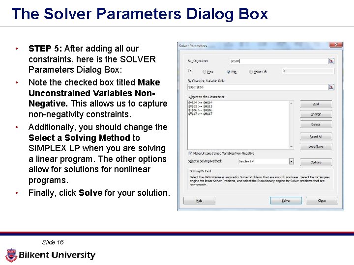
The Solver Parameters Dialog Box • • STEP 5: After adding all our constraints, here is the SOLVER Parameters Dialog Box: Note the checked box titled Make Unconstrained Variables Non. Negative. This allows us to capture non-negativity constraints. Additionally, you should change the Select a Solving Method to SIMPLEX LP when you are solving a linear program. The other options allow for solutions for nonlinear programs. Finally, click Solve for your solution. Slide 16

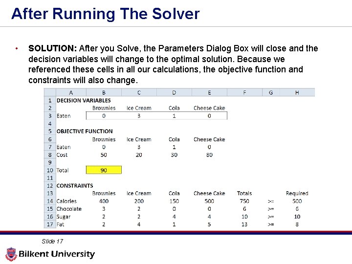
After Running The Solver • SOLUTION: After you Solve, the Parameters Dialog Box will close and the decision variables will change to the optimal solution. Because we referenced these cells in all our calculations, the objective function and constraints will also change. Slide 17

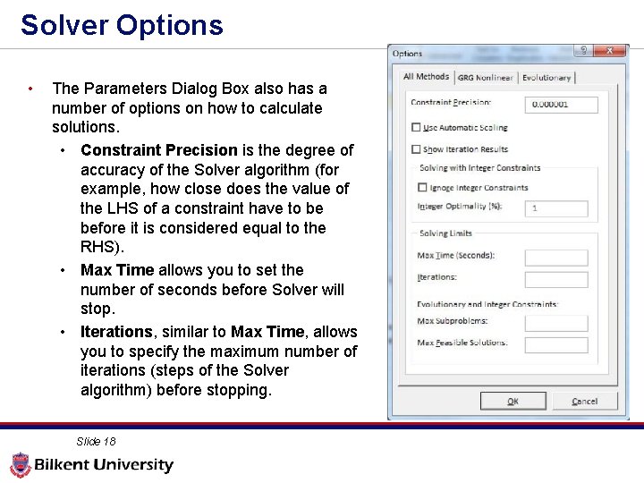
Solver Options • The Parameters Dialog Box also has a number of options on how to calculate solutions. • Constraint Precision is the degree of accuracy of the Solver algorithm (for example, how close does the value of the LHS of a constraint have to be before it is considered equal to the RHS). • Max Time allows you to set the number of seconds before Solver will stop. • Iterations, similar to Max Time, allows you to specify the maximum number of iterations (steps of the Solver algorithm) before stopping. Slide 18

Limits of the Solver • You may have at most 200 decision variables and 100 constraints! • For any decision variables or constraints above these limits will disable solver! • You can download and use Open. Solver (opensolver. org) for large models. • It has a very similar structure but more capabilities. Slide 19

Example • Go to the Excel Sheet. . . Slide 20