EvaluationInterpolation II Lecture 8 Richard Fateman CS 282

Evaluation/Interpolation (II) Lecture 8 Richard Fateman CS 282 Lecture 8 1

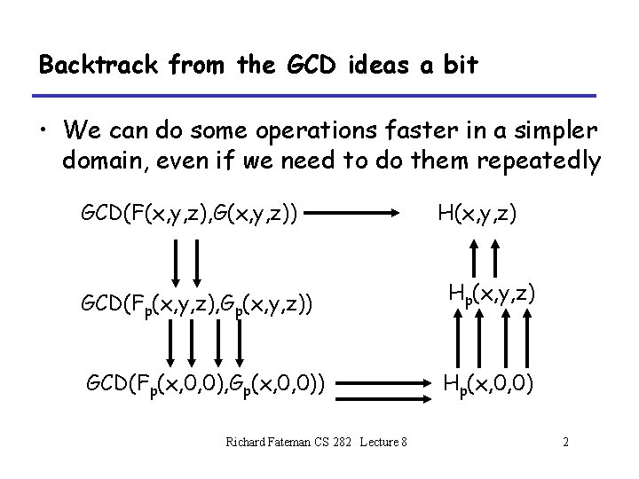
Backtrack from the GCD ideas a bit • We can do some operations faster in a simpler domain, even if we need to do them repeatedly GCD(F(x, y, z), G(x, y, z)) H(x, y, z) GCD(Fp(x, y, z), Gp(x, y, z)) Hp(x, y, z) GCD(Fp(x, 0, 0), Gp(x, 0, 0)) Hp(x, 0, 0) Richard Fateman CS 282 Lecture 8 2

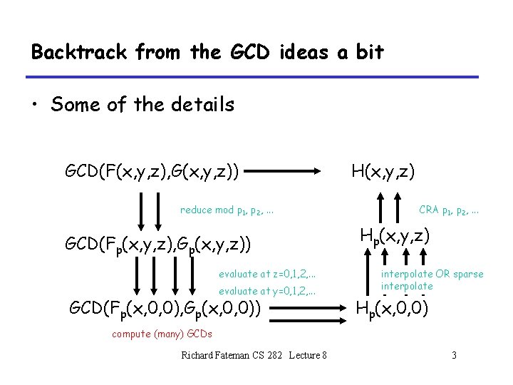
Backtrack from the GCD ideas a bit • Some of the details GCD(F(x, y, z), G(x, y, z)) reduce mod p 1, p 2, . . . GCD(Fp(x, y, z), Gp(x, y, z)) evaluate at z=0, 1, 2, . . . evaluate at y=0, 1, 2, . . . GCD(Fp(x, 0, 0), Gp(x, 0, 0)) H(x, y, z) CRA p 1, p 2, . . . Hp(x, y, z) interpolate OR sparse interpolate Hp(x, 0, 0) compute (many) GCDs Richard Fateman CS 282 Lecture 8 3

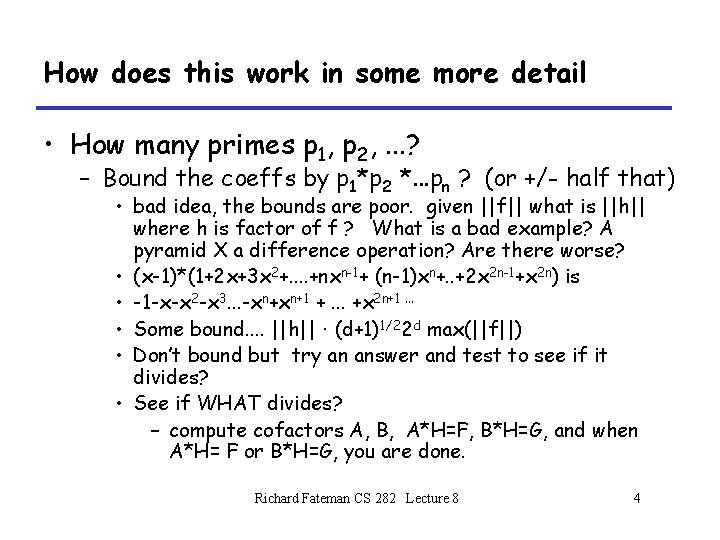
How does this work in some more detail • How many primes p 1, p 2, . . . ? – Bound the coeffs by p 1*p 2 *. . . pn ? (or +/- half that) • bad idea, the bounds are poor. given ||f|| what is ||h|| where h is factor of f ? What is a bad example? A pyramid X a difference operation? Are there worse? • (x-1)*(1+2 x+3 x 2+. . +nxn-1+ (n-1)xn+. . +2 x 2 n-1+x 2 n) is • -1 -x-x 2 -x 3. . . -xn+xn+1 +. . . +x 2 n+1. . . • Some bound. . ||h|| · (d+1)1/22 d max(||f||) • Don’t bound but try an answer and test to see if it divides? • See if WHAT divides? – compute cofactors A, B, A*H=F, B*H=G, and when A*H= F or B*H=G, you are done. Richard Fateman CS 282 Lecture 8 4

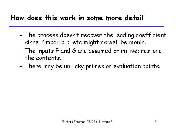
How does this work in some more detail – The process doesn’t recover the leading coefficient since F modulo p etc might as well be monic. – The inputs F and G are assumed primitive; restore the contents. – There may be unlucky primes or evaluation points. Richard Fateman CS 282 Lecture 8 5

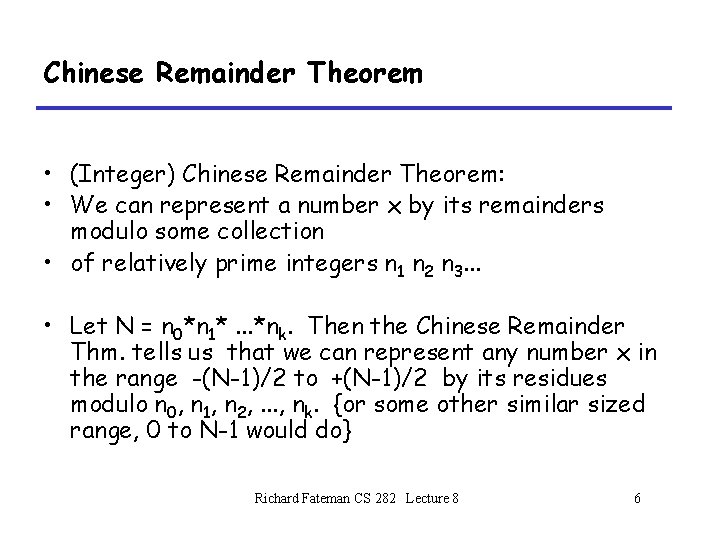
Chinese Remainder Theorem • (Integer) Chinese Remainder Theorem: • We can represent a number x by its remainders modulo some collection • of relatively prime integers n 1 n 2 n 3. . . • Let N = n 0*n 1*. . . *nk. Then the Chinese Remainder Thm. tells us that we can represent any number x in the range -(N-1)/2 to +(N-1)/2 by its residues modulo n 0, n 1, n 2, . . . , nk. {or some other similar sized range, 0 to N-1 would do} Richard Fateman CS 282 Lecture 8 6

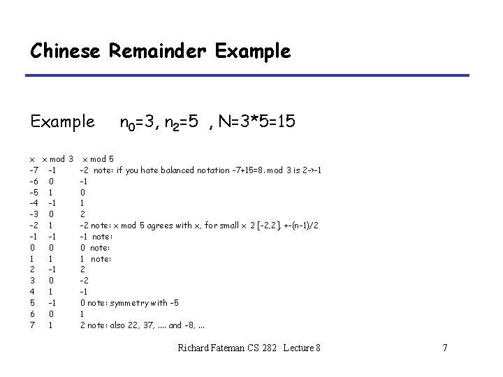
Chinese Remainder Example x x mod 3 -7 -1 -6 0 -5 1 -4 -1 -3 0 -2 1 -1 -1 0 0 1 1 2 -1 3 0 4 1 5 -1 6 0 7 1 n 0=3, n 2=5 , N=3*5=15 x mod 5 -2 note: if you hate balanced notation -7+15=8. mod 3 is 2 ->-1 -1 0 1 2 -2 note: x mod 5 agrees with x, for small x 2 [-2, 2], +-(n-1)/2 -1 note: 0 note: 1 note: 2 -2 -1 0 note: symmetry with -5 1 2 note: also 22, 37, . . and -8, . . . Richard Fateman CS 282 Lecture 8 7

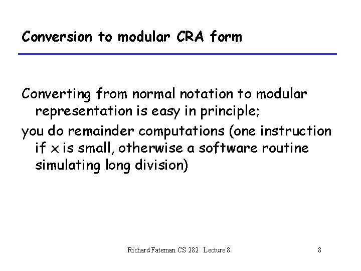
Conversion to modular CRA form Converting from normal notation to modular representation is easy in principle; you do remainder computations (one instruction if x is small, otherwise a software routine simulating long division) Richard Fateman CS 282 Lecture 8 8

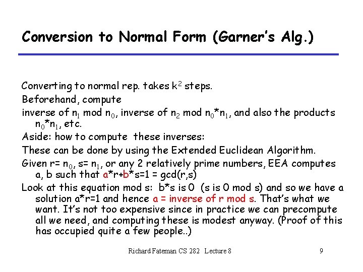
Conversion to Normal Form (Garner’s Alg. ) Converting to normal rep. takes k 2 steps. Beforehand, compute inverse of n 1 mod n 0, inverse of n 2 mod n 0*n 1, and also the products n 0*n 1, etc. Aside: how to compute these inverses: These can be done by using the Extended Euclidean Algorithm. Given r= n 0, s= n 1, or any 2 relatively prime numbers, EEA computes a, b such that a*r+b*s=1 = gcd(r, s) Look at this equation mod s: b*s is 0 (s is 0 mod s) and so we have a solution a*r=1 and hence a = inverse of r mod s. That’s what we want. It’s not too expensive since in practice we can precompute all we need, and computing these is modest anyway. (Proof of this has occupied quite a few people. . ) Richard Fateman CS 282 Lecture 8 9

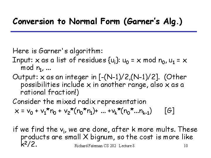
Conversion to Normal Form (Garner’s Alg. ) Here is Garner's algorithm: Input: x as a list of residues {ui}: u 0 = x mod n 0, u 1 = x mod n 1, . . . Output: x as an integer in [-(N-1)/2, (N-1)/2]. (Other possibilities include x in another range, also x as a rational fraction!) Consider the mixed radix representation x = v 0 + v 1*n 0 + v 2*(n 0*n 1)+. . . +vk*(n 0*. . . nk-1) [G] if we find the vi, we are done, after k more mults. These products are small X bignum, so the cost is more like k 2/2. Richard Fateman CS 282 Lecture 8 10

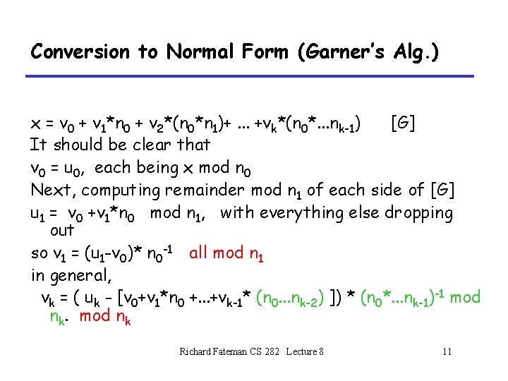
Conversion to Normal Form (Garner’s Alg. ) x = v 0 + v 1*n 0 + v 2*(n 0*n 1)+. . . +vk*(n 0*. . . nk-1) [G] It should be clear that v 0 = u 0, each being x mod n 0 Next, computing remainder mod n 1 of each side of [G] u 1 = v 0 +v 1*n 0 mod n 1, with everything else dropping out so v 1 = (u 1 -v 0)* n 0 -1 all mod n 1 in general, vk = ( uk - [v 0+v 1*n 0 +. . . +vk-1* (n 0. . . nk-2) ]) * (n 0*. . . nk-1)-1 mod nk Richard Fateman CS 282 Lecture 8 11

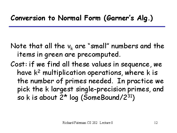
Conversion to Normal Form (Garner’s Alg. ) Note that all the vk are “small” numbers and the items in green are precomputed. Cost: if we find all these values in sequence, we have k 2 multiplication operations, where k is the number of primes needed. In practice we pick the k largest single-precision primes, and so k is about 2* log (Some. Bound/231) Richard Fateman CS 282 Lecture 8 12

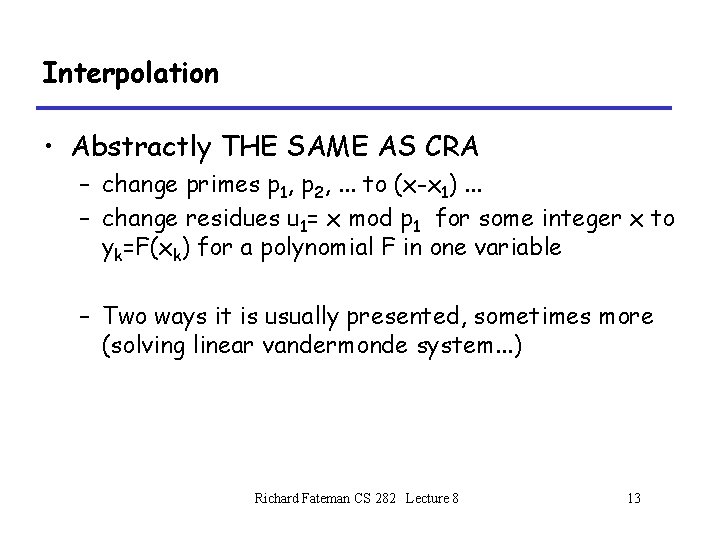
Interpolation • Abstractly THE SAME AS CRA – change primes p 1, p 2, . . . to (x-x 1). . . – change residues u 1= x mod p 1 for some integer x to yk=F(xk) for a polynomial F in one variable – Two ways it is usually presented, sometimes more (solving linear vandermonde system. . . ) Richard Fateman CS 282 Lecture 8 13

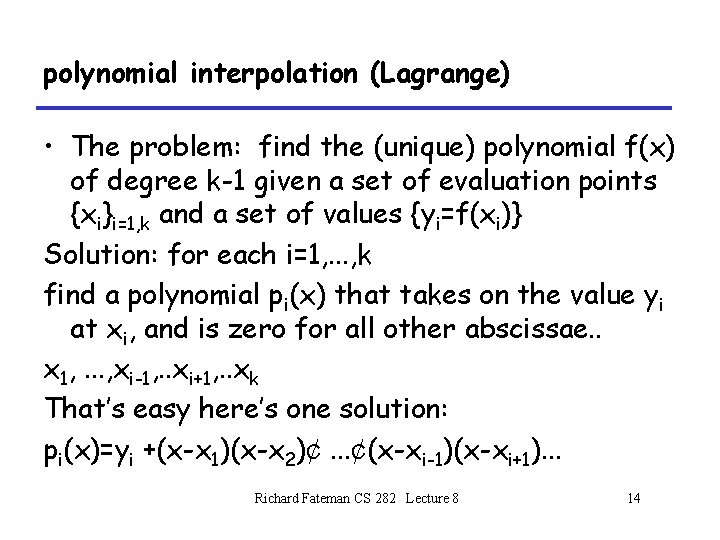
polynomial interpolation (Lagrange) • The problem: find the (unique) polynomial f(x) of degree k-1 given a set of evaluation points {xi}i=1, k and a set of values {yi=f(xi)} Solution: for each i=1, . . . , k find a polynomial pi(x) that takes on the value yi at xi, and is zero for all other abscissae. . x 1, . . . , xi-1, . . xi+1, . . xk That’s easy here’s one solution: pi(x)=yi +(x-x 1)(x-x 2)¢. . . ¢(x-xi-1)(x-xi+1). . . Richard Fateman CS 282 Lecture 8 14

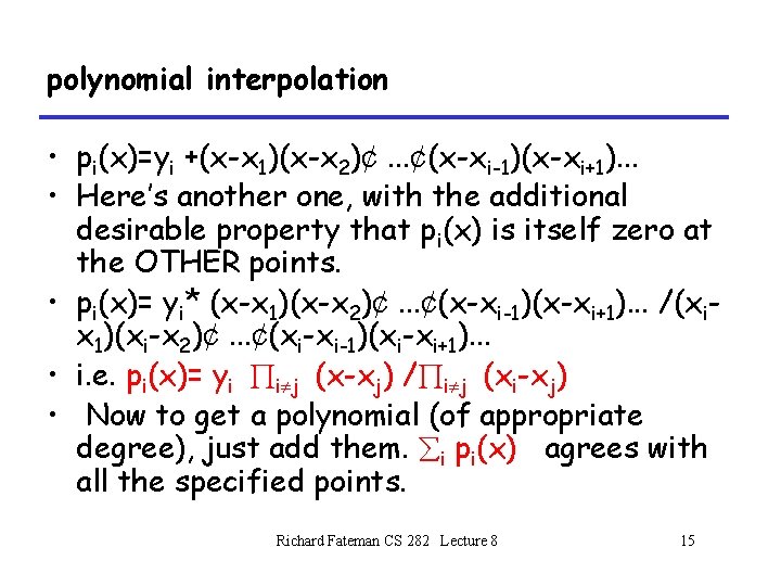
polynomial interpolation • pi(x)=yi +(x-x 1)(x-x 2)¢. . . ¢(x-xi-1)(x-xi+1). . . • Here’s another one, with the additional desirable property that pi(x) is itself zero at the OTHER points. • pi(x)= yi* (x-x 1)(x-x 2)¢. . . ¢(x-xi-1)(x-xi+1). . . /(xix 1)(xi-x 2)¢. . . ¢(xi-xi-1)(xi-xi+1). . . • i. e. pi(x)= yi Õi j (x-xj) /Õi j (xi-xj) • Now to get a polynomial (of appropriate degree), just add them. åi pi(x) agrees with all the specified points. Richard Fateman CS 282 Lecture 8 15

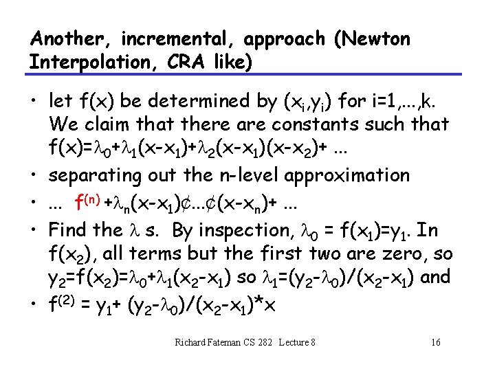
Another, incremental, approach (Newton Interpolation, CRA like) • let f(x) be determined by (xi, yi) for i=1, . . . , k. We claim that there are constants such that f(x)=l 0+l 1(x-x 1)+l 2(x-x 1)(x-x 2)+. . . • separating out the n-level approximation • . . . f(n) +ln(x-x 1)¢. . . ¢(x-xn)+. . . • Find the l s. By inspection, l 0 = f(x 1)=y 1. In f(x 2), all terms but the first two are zero, so y 2=f(x 2)=l 0+l 1(x 2 -x 1) so l 1=(y 2 -l 0)/(x 2 -x 1) and • f(2) = y 1+ (y 2 -l 0)/(x 2 -x 1)*x Richard Fateman CS 282 Lecture 8 16

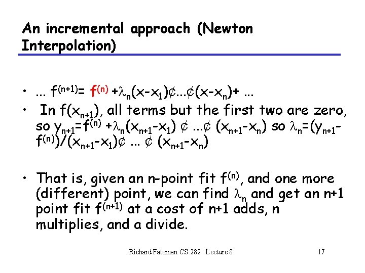
An incremental approach (Newton Interpolation) • . . . f(n+1)= f(n) +ln(x-x 1)¢. . . ¢(x-xn)+. . . • In f(xn+1), all terms but the first two are zero, so yn+1=f(n) +ln(xn+1 -x 1) ¢. . . ¢ (xn+1 -xn) so ln=(yn+1 f(n))/(xn+1 -x 1)¢. . . ¢ (xn+1 -xn) • That is, given an n-point fit f(n), and one more (different) point, we can find ln and get an n+1 point fit f(n+1) at a cost of n+1 adds, n multiplies, and a divide. Richard Fateman CS 282 Lecture 8 17

polynomial interpolation • Additional notes. The Lagrange and Newton forms of interpolation are effectively the same, with an identical computation with different order of operations: • Note that yi can, without loss of generality, be a polynomial in other variables. Richard Fateman CS 282 Lecture 8 18

Sparse Multivariate Interpolation • There is a better way to do interpolation if you think that the number of terms in the answer is much lower than the degree, and you have several variables. (R. Zippel) Richard Fateman CS 282 Lecture 8 19

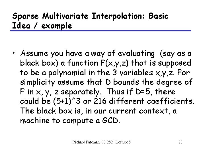
Sparse Multivariate Interpolation: Basic Idea / example • Assume you have a way of evaluating (say as a black box) a function F(x, y, z) that is supposed to be a polynomial in the 3 variables x, y, z. For simplicity assume that D bounds the degree of F in x, y, z separately. Thus if D=5, there could be (5+1)^3 or 216 different coefficients. The black box is, in our current context, a machine to compute a GCD. Richard Fateman CS 282 Lecture 8 20

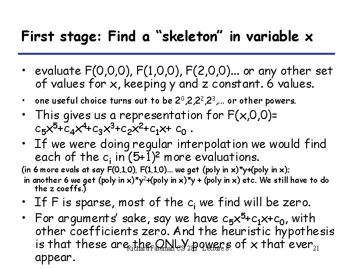
First stage: Find a “skeleton” in variable x • evaluate F(0, 0, 0), F(1, 0, 0), F(2, 0, 0). . . or any other set of values for x, keeping y and z constant. 6 values. • one useful choice turns out to be 20, 2, 23, . . . or other powers. • This gives us a representation for F(x, 0, 0)= c 5 x 5+c 4 x 4+c 3 x 3+c 2 x 2+c 1 x+ c 0. • If we were doing regular interpolation we would find each of the ci in (5+1)2 more evaluations. (in 6 more evals at say F(0, 1, 0), F(1, 1, 0). . . we get (poly in x)*y+(poly in x); in another 6 we get (poly in x)*y 2+(poly in x)*y + (poly in x) etc. We still have to do the z coeffs. ) • If F is sparse, most of the ci we find will be zero. • For arguments’ sake, say we have c 5 x 5+c 1 x+c 0, with other coefficients zero. And the heuristic hypothesis is that these are. Richard the. Fateman ONLY powers CS 282 Lecture 8 of x that ever 21 appear.

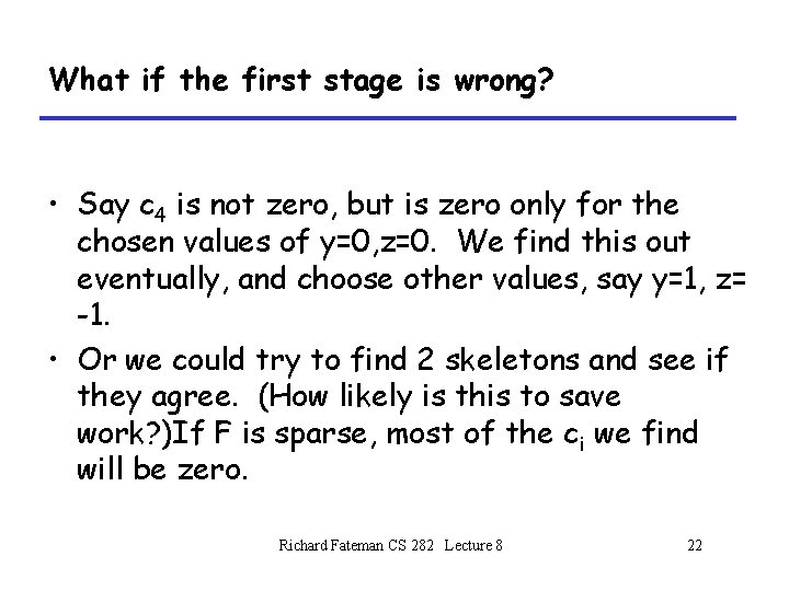
What if the first stage is wrong? • Say c 4 is not zero, but is zero only for the chosen values of y=0, z=0. We find this out eventually, and choose other values, say y=1, z= -1. • Or we could try to find 2 skeletons and see if they agree. (How likely is this to save work? )If F is sparse, most of the ci we find will be zero. Richard Fateman CS 282 Lecture 8 22

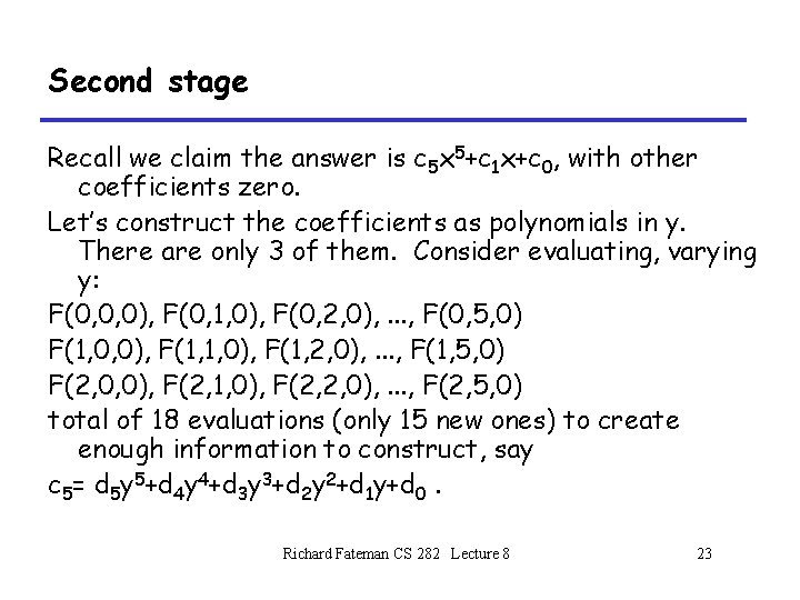
Second stage Recall we claim the answer is c 5 x 5+c 1 x+c 0, with other coefficients zero. Let’s construct the coefficients as polynomials in y. There are only 3 of them. Consider evaluating, varying y: F(0, 0, 0), F(0, 1, 0), F(0, 2, 0), . . . , F(0, 5, 0) F(1, 0, 0), F(1, 1, 0), F(1, 2, 0), . . . , F(1, 5, 0) F(2, 0, 0), F(2, 1, 0), F(2, 2, 0), . . . , F(2, 5, 0) total of 18 evaluations (only 15 new ones) to create enough information to construct, say c 5= d 5 y 5+d 4 y 4+d 3 y 3+d 2 y 2+d 1 y+d 0. Richard Fateman CS 282 Lecture 8 23

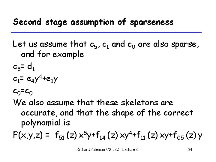
Second stage assumption of sparseness Let us assume that c 5, c 1 and c 0 are also sparse, and for example c 5= d 1 c 1= e 4 y 4+e 1 y c 0=c 0 We also assume that these skeletons are accurate, and that the shape of the correct polynomial is F(x, y, z) = f 51 (z) x 5 y+f 14 (z) xy 4+f 11 (z) xy+f 05 (z) y Richard Fateman CS 282 Lecture 8 24

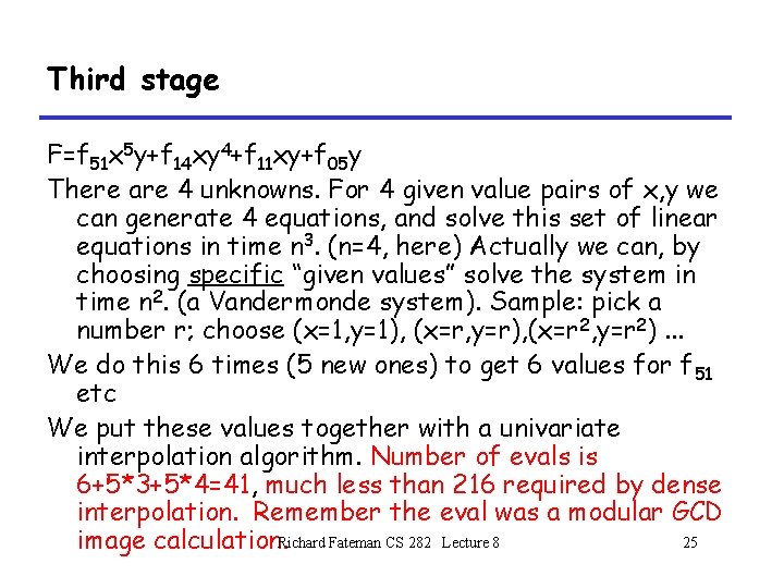
Third stage F=f 51 x 5 y+f 14 xy 4+f 11 xy+f 05 y There are 4 unknowns. For 4 given value pairs of x, y we can generate 4 equations, and solve this set of linear equations in time n 3. (n=4, here) Actually we can, by choosing specific “given values” solve the system in time n 2. (a Vandermonde system). Sample: pick a number r; choose (x=1, y=1), (x=r, y=r), (x=r 2, y=r 2). . . We do this 6 times (5 new ones) to get 6 values for f 51 etc We put these values together with a univariate interpolation algorithm. Number of evals is 6+5*3+5*4=41, much less than 216 required by dense interpolation. Remember the eval was a modular GCD 25 image calculation. Richard Fateman CS 282 Lecture 8

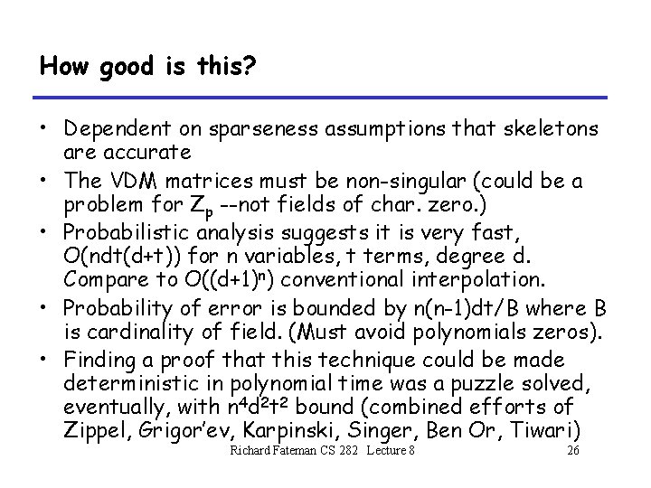
How good is this? • Dependent on sparseness assumptions that skeletons are accurate • The VDM matrices must be non-singular (could be a problem for Zp --not fields of char. zero. ) • Probabilistic analysis suggests it is very fast, O(ndt(d+t)) for n variables, t terms, degree d. Compare to O((d+1)n) conventional interpolation. • Probability of error is bounded by n(n-1)dt/B where B is cardinality of field. (Must avoid polynomials zeros). • Finding a proof that this technique could be made deterministic in polynomial time was a puzzle solved, eventually, with n 4 d 2 t 2 bound (combined efforts of Zippel, Grigor’ev, Karpinski, Singer, Ben Or, Tiwari) Richard Fateman CS 282 Lecture 8 26

Polynomial evaluation • What’s to say? Richard Fateman CS 282 Lecture 8 27

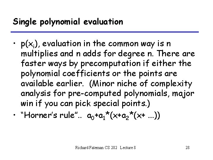
Single polynomial evaluation • p(xi), evaluation in the common way is n multiplies and n adds for degree n. There are faster ways by precomputation if either the polynomial coefficients or the points are available earlier. (Minor niche of complexity analysis for pre-computed polynomials, major win if you can pick special points. ) • “Horner’s rule”. . a 0+a 1*(x+a 2*(x+. . . )) Richard Fateman CS 282 Lecture 8 28

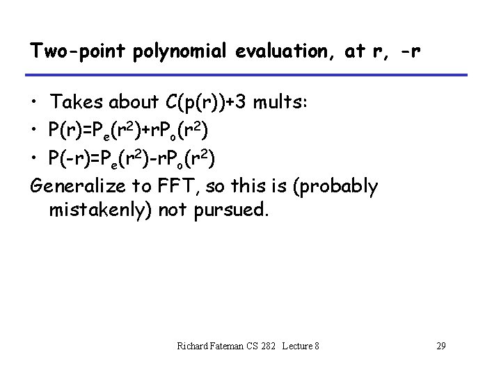
Two-point polynomial evaluation, at r, -r • Takes about C(p(r))+3 mults: • P(r)=Pe(r 2)+r. Po(r 2) • P(-r)=Pe(r 2)-r. Po(r 2) Generalize to FFT, so this is (probably mistakenly) not pursued. Richard Fateman CS 282 Lecture 8 29

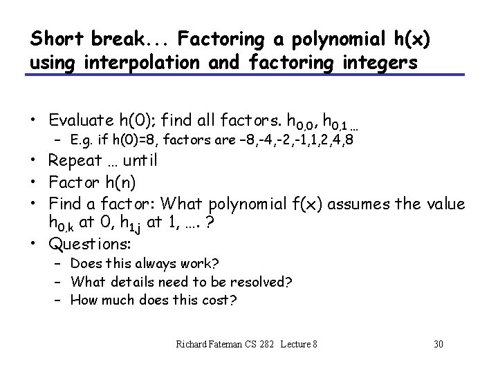
Short break. . . Factoring a polynomial h(x) using interpolation and factoring integers • Evaluate h(0); find all factors. h 0, 0, h 0, 1 … – E. g. if h(0)=8, factors are – 8, -4, -2, -1, 1, 2, 4, 8 • Repeat … until • Factor h(n) • Find a factor: What polynomial f(x) assumes the value h 0, k at 0, h 1, j at 1, …. ? • Questions: – Does this always work? – What details need to be resolved? – How much does this cost? Richard Fateman CS 282 Lecture 8 30

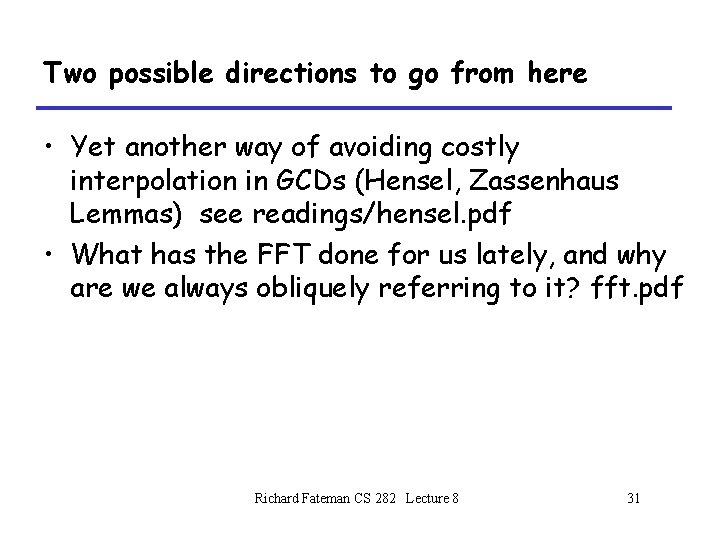
Two possible directions to go from here • Yet another way of avoiding costly interpolation in GCDs (Hensel, Zassenhaus Lemmas) see readings/hensel. pdf • What has the FFT done for us lately, and why are we always obliquely referring to it? fft. pdf Richard Fateman CS 282 Lecture 8 31