Estimators For Extracting Primordial NonGaussianity Eiichiro Komatsu University

Estimators For Extracting (Primordial) Non-Gaussianity Eiichiro Komatsu University of Texas, Austin June 8, 2007

Why Study NG? (Why Care? !) n Who said that CMB should be Gaussian? n n n Don’t let people take it for granted! It is remarkable that the observed CMB is (very close to being) Gaussian. The WMAP map, when smoothed to 1 degree, is entirely dominated by the CMB signal. • If it were still noise dominated, no one would be surprised that the map is Gaussian. n The WMAP data are telling us that primordial fluctuations are very close to being Gaussian. • How common is it to have something so close to being Gaussian in astronomy? E. g. , Maxwellian velocity distribution, what else? n It may not be so easy to explain that CMB is Gaussian, unless we have a compelling early universe model that predicts Gaussian primordial fluctuations: Inflation. A strong theoretical prior! n “Gaussianity” should be taken as seriously as “Flatness”.

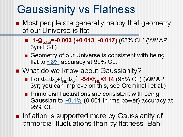
Gaussianity vs Flatness n Most people are generally happy that geometry of our Universe is flat. n 1 -Wtotal=-0. 003 (+0. 013, -0. 017) (68% CL) (WMAP n n What do we know about Gaussianity? n n n 3 yr+HST) Geometry of our Universe is consistent with being flat to ~3% accuracy at 95% CL. For = G+f. NL G 2, -54<f. NL<114 (95% CL) (WMAP 3 yr; you can improve on this, see Creminelli et al. ) Primordial fluctuations are consistent with being Gaussian to ~0. 1% (0. 001 in rms power) accuracy at 95% CL. Inflation is supported more by Gaussianity of primordial fluctuations than by flatness. Bah!

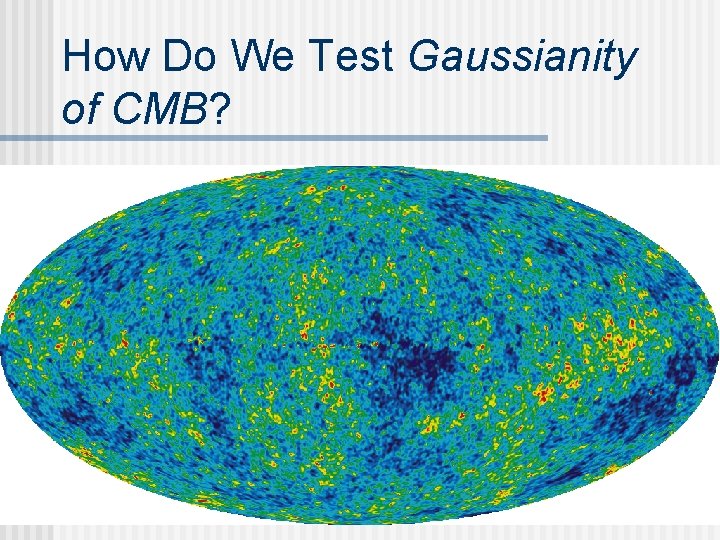
How Do We Test Gaussianity of CMB?

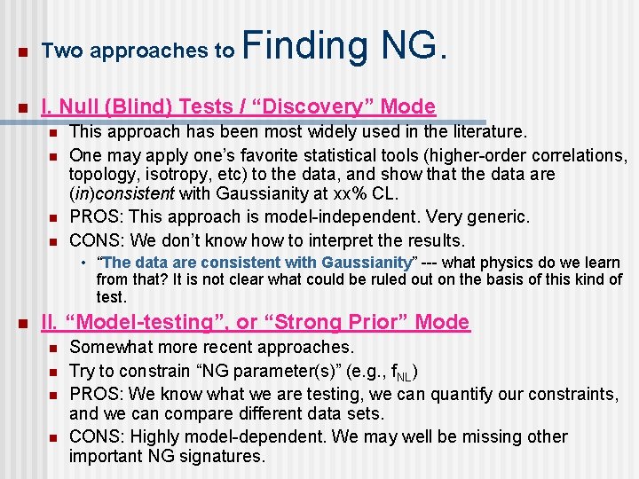
Finding NG. n Two approaches to n I. Null (Blind) Tests / “Discovery” Mode n n This approach has been most widely used in the literature. One may apply one’s favorite statistical tools (higher-order correlations, topology, isotropy, etc) to the data, and show that the data are (in)consistent with Gaussianity at xx% CL. PROS: This approach is model-independent. Very generic. CONS: We don’t know how to interpret the results. • “The data are consistent with Gaussianity” --- what physics do we learn from that? It is not clear what could be ruled out on the basis of this kind of test. n II. “Model-testing”, or “Strong Prior” Mode n n Somewhat more recent approaches. Try to constrain “NG parameter(s)” (e. g. , f. NL) PROS: We know what we are testing, we can quantify our constraints, and we can compare different data sets. CONS: Highly model-dependent. We may well be missing other important NG signatures.

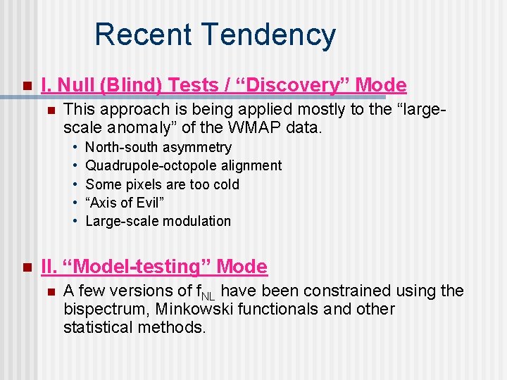
Recent Tendency n I. Null (Blind) Tests / “Discovery” Mode n This approach is being applied mostly to the “largescale anomaly” of the WMAP data. • • • n North-south asymmetry Quadrupole-octopole alignment Some pixels are too cold “Axis of Evil” Large-scale modulation II. “Model-testing” Mode n A few versions of f. NL have been constrained using the bispectrum, Minkowski functionals and other statistical methods.

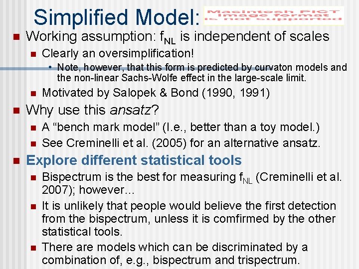
Simplified Model: n Working assumption: f. NL is independent of scales n Clearly an oversimplification! • Note, however, that this form is predicted by curvaton models and the non-linear Sachs-Wolfe effect in the large-scale limit. n n Why use this ansatz? n n n Motivated by Salopek & Bond (1990, 1991) A “bench mark model” (I. e. , better than a toy model. ) See Creminelli et al. (2005) for an alternative ansatz. Explore different statistical tools n n n Bispectrum is the best for measuring f. NL (Creminelli et al. 2007); however… It is unlikely that people would believe the first detection from the bispectrum, unless it is comfirmed by the other statistical tools. There are models which can be discriminated by a combination of, e. g. , bispectrum and trispectrum.

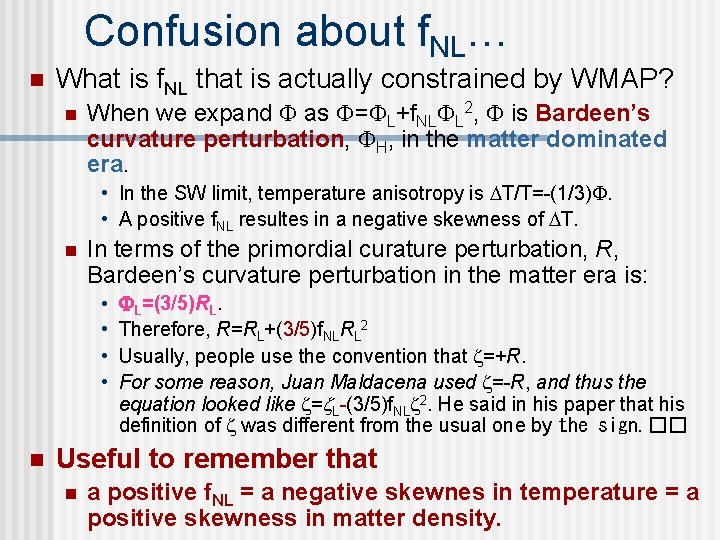
Confusion about f. NL… n What is f. NL that is actually constrained by WMAP? n When we expand as = L+f. NL L 2, is Bardeen’s curvature perturbation, H, in the matter dominated era. • In the SW limit, temperature anisotropy is T/T=-(1/3). • A positive f. NL resultes in a negative skewness of T. n In terms of the primordial curature perturbation, R, Bardeen’s curvature perturbation in the matter era is: • • n L=(3/5)RL. Therefore, R=RL+(3/5)f. NLRL 2 Usually, people use the convention that =+R. For some reason, Juan Maldacena used =-R, and thus the equation looked like = L-(3/5)f. NL 2. He said in his paper that his definition of was different from the usual one by the sign. �� Useful to remember that n a positive f. NL = a negative skewnes in temperature = a positive skewness in matter density.

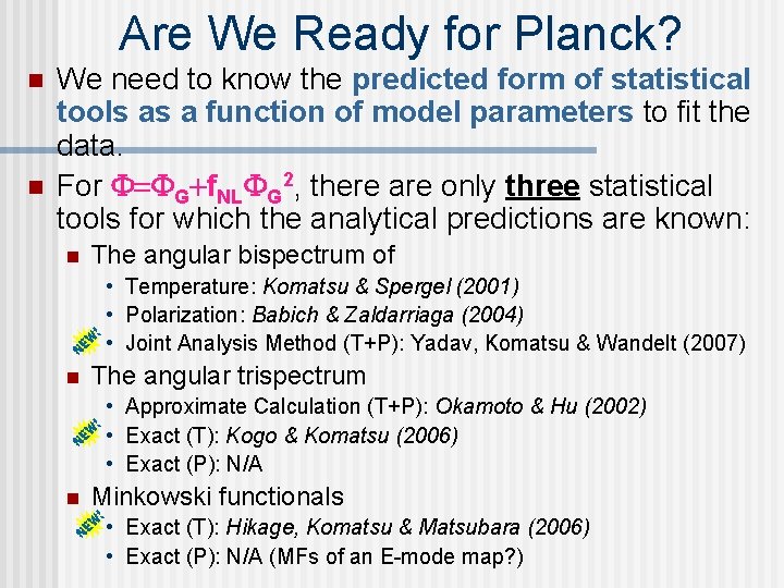
Are We Ready for Planck? n n We need to know the predicted form of statistical tools as a function of model parameters to fit the data. For = G+f. NL G 2, there are only three statistical tools for which the analytical predictions are known: n The angular bispectrum of • Temperature: Komatsu & Spergel (2001) • Polarization: Babich & Zaldarriaga (2004) • Joint Analysis Method (T+P): Yadav, Komatsu & Wandelt (2007) n The angular trispectrum • Approximate Calculation (T+P): Okamoto & Hu (2002) • Exact (T): Kogo & Komatsu (2006) • Exact (P): N/A n Minkowski functionals • Exact (T): Hikage, Komatsu & Matsubara (2006) • Exact (P): N/A (MFs of an E-mode map? )

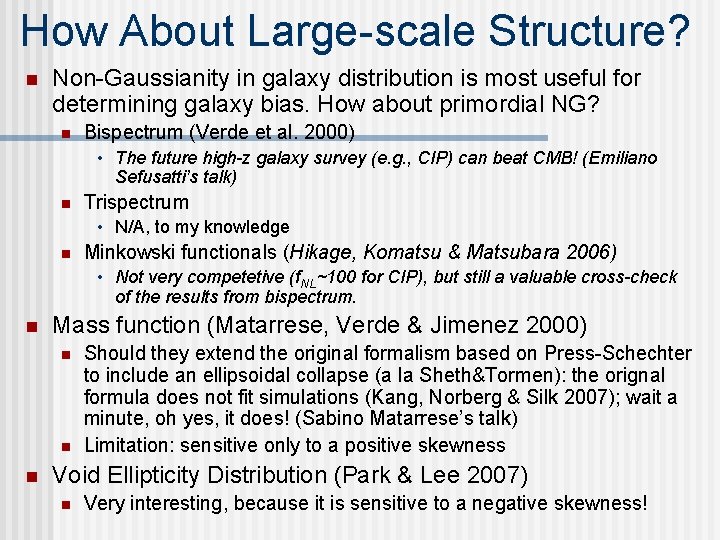
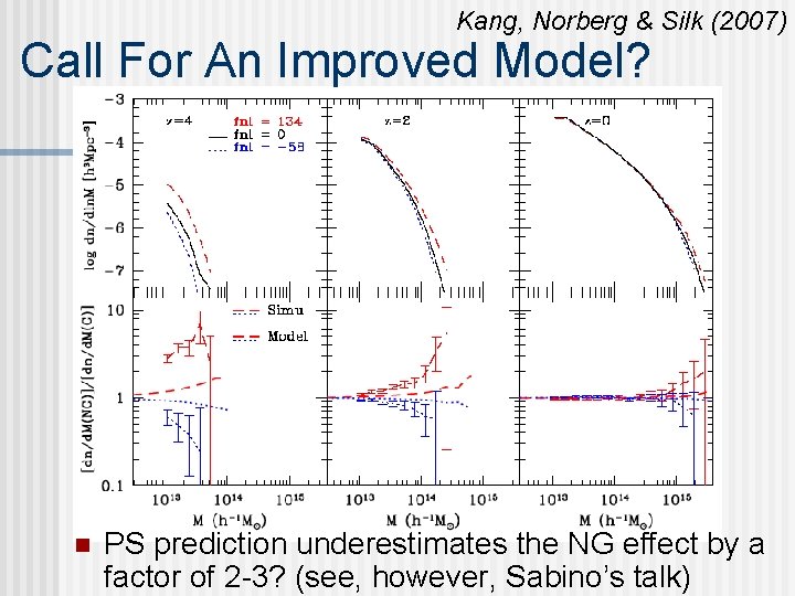
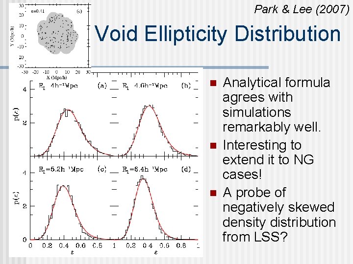
How About Large-scale Structure? n Non-Gaussianity in galaxy distribution is most useful for determining galaxy bias. How about primordial NG? n Bispectrum (Verde et al. 2000) • The future high-z galaxy survey (e. g. , CIP) can beat CMB! (Emiliano Sefusatti’s talk) n Trispectrum • N/A, to my knowledge n Minkowski functionals (Hikage, Komatsu & Matsubara 2006) • Not very competetive (f. NL~100 for CIP), but still a valuable cross-check of the results from bispectrum. n Mass function (Matarrese, Verde & Jimenez 2000) n n n Should they extend the original formalism based on Press-Schechter to include an ellipsoidal collapse (a la Sheth&Tormen): the orignal formula does not fit simulations (Kang, Norberg & Silk 2007); wait a minute, oh yes, it does! (Sabino Matarrese’s talk) Limitation: sensitive only to a positive skewness Void Ellipticity Distribution (Park & Lee 2007) n Very interesting, because it is sensitive to a negative skewness!

Kang, Norberg & Silk (2007) Call For An Improved Model? n PS prediction underestimates the NG effect by a factor of 2 -3? (see, however, Sabino’s talk)

Park & Lee (2007) Void Ellipticity Distribution n Analytical formula agrees with simulations remarkably well. Interesting to extend it to NG cases! A probe of negatively skewed density distribution from LSS?

Ingredient: Probability Distribution of the Eigenvalues of the Tidal Tensor n Eigenvalues of the tidal tenspr: n n Probability distribution of from a Gassian field is given analytically by Doroshkevich (1970). n n Tidal tensor = ij To do: obtain the distribution of from a non-Gaussian field (e. g. , f. NL) Straightforward, and unique.

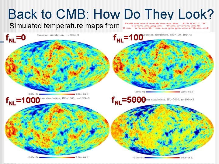
Back to CMB: How Do They Look? Simulated temperature maps from f. NL=0 f. NL=1000 f. NL=5000

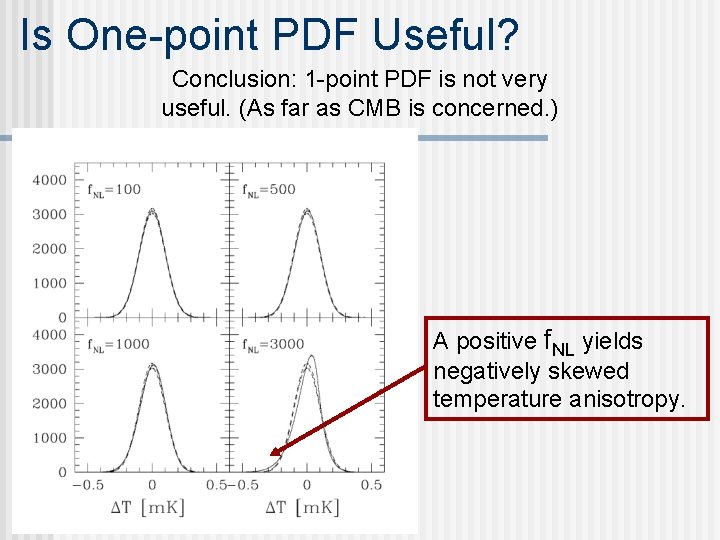
Is One-point PDF Useful? Conclusion: 1 -point PDF is not very useful. (As far as CMB is concerned. ) A positive f. NL yields negatively skewed temperature anisotropy.

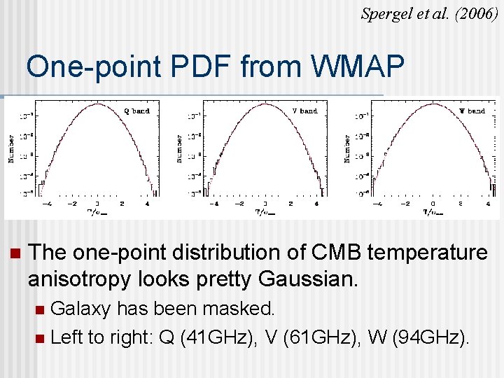
Spergel et al. (2006) One-point PDF from WMAP n The one-point distribution of CMB temperature anisotropy looks pretty Gaussian. Galaxy has been masked. n Left to right: Q (41 GHz), V (61 GHz), W (94 GHz). n

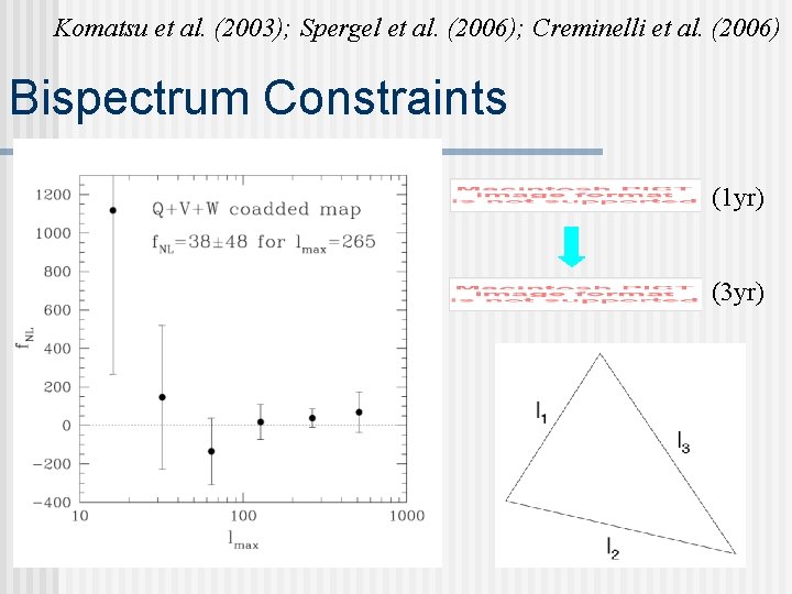
Komatsu et al. (2003); Spergel et al. (2006); Creminelli et al. (2006) Bispectrum Constraints (1 yr) (3 yr)

How do we measure f. NL from Planck? n Good News! We are now ready to use both the temperature and polarization data from Planck to measure f. NL. n Amit Yadav, EK�� & Wandelt Ben (2007 a, b) n Amit’s code is “Planck-ready”. n n Stay tuned for Ben Wandelt’s talk.

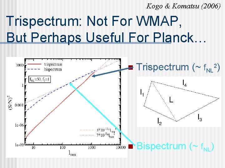
Kogo & Komatsu (2006) Trispectrum: Not For WMAP, But Perhaps Useful For Planck… n Trispectrum (~ f. NL 2) n Bispectrum (~ f. NL)

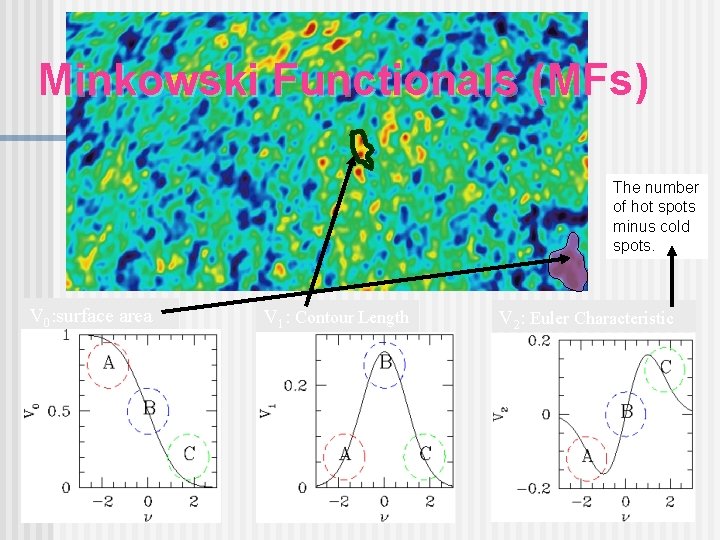
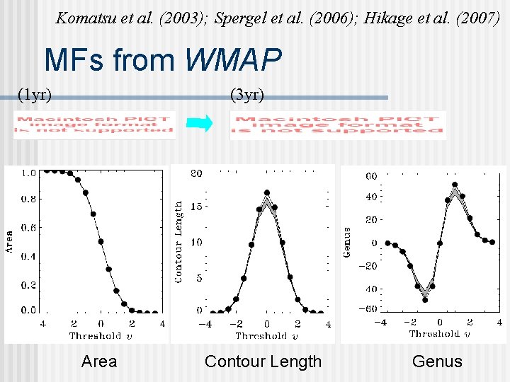
Minkowski Functionals (MFs) The number of hot spots minus cold spots. V 0: surface area V 1: Contour Length V 2: Euler Characteristic

Komatsu et al. (2003); Spergel et al. (2006); Hikage et al. (2007) MFs from WMAP (1 yr) (3 yr) Area Contour Length Genus

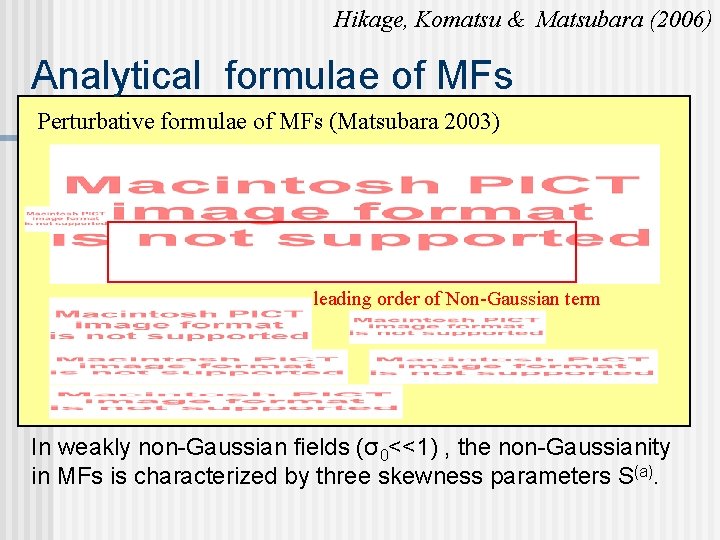
Hikage, Komatsu & Matsubara (2006) Analytical formulae of MFs Perturbative formulae of MFs (Matsubara 2003) Gaussian term leading order of Non-Gaussian term In weakly non-Gaussian fields (σ0<<1) , the non-Gaussianity in MFs is characterized by three skewness parameters S(a).

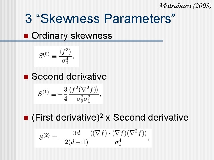
Matsubara (2003) 3 “Skewness Parameters” n Ordinary skewness n Second derivative n (First derivative)2 x Second derivative

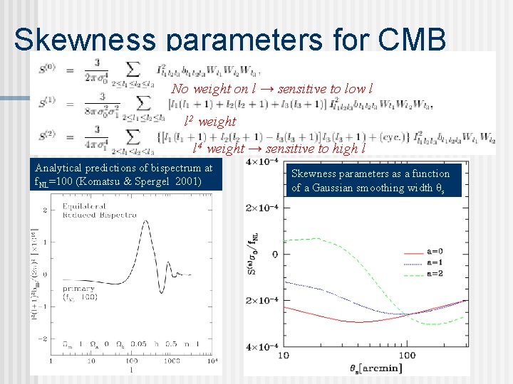
Skewness parameters for CMB No weight on l → sensitive to low l l 2 weight l 4 weight → sensitive to high l Analytical predictions of bispectrum at f. NL=100 (Komatsu & Spergel 2001) Skewness parameters as a function of a Gaussian smoothing width θs

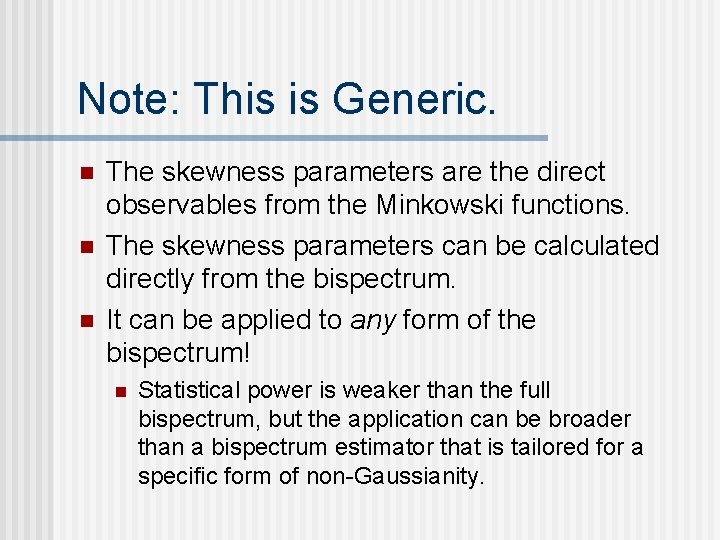
Note: This is Generic. n n n The skewness parameters are the direct observables from the Minkowski functions. The skewness parameters can be calculated directly from the bispectrum. It can be applied to any form of the bispectrum! n Statistical power is weaker than the full bispectrum, but the application can be broader than a bispectrum estimator that is tailored for a specific form of non-Gaussianity.

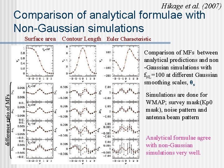
Hikage et al. (2007) Comparison of analytical formulae with Non-Gaussian simulations Surface area Contour Length Euler Characteristic difference ratio of MFs Comparison of MFs between analytical predictions and non -Gaussian simulations with f. NL=100 at different Gaussian smoothing scales, θs Simulations are done for WMAP; survey mask(Kp 0 mask), noise pattern and antenna beam pattern Analytical formulae agree with non-Gaussian simulations very well.

How do we measure f. NL from Planck? n Good News! We are now ready to measure f. NL from Planck with the Minkowski Functionals. n Chiaki Hikage, EK, et al. (2006, 2007) n • A postdoc at the Univ. of Nottingham. n Chiaki’s code is “Planck-ready”.

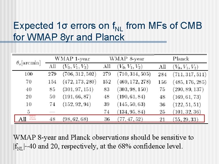
Expected 1σ errors on f. NL from MFs of CMB for WMAP 8 yr and Planck All WMAP 8 -year and Planck observations should be sensitive to |f. NL|~40 and 20, respectively, at the 68% confidence level.

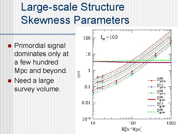
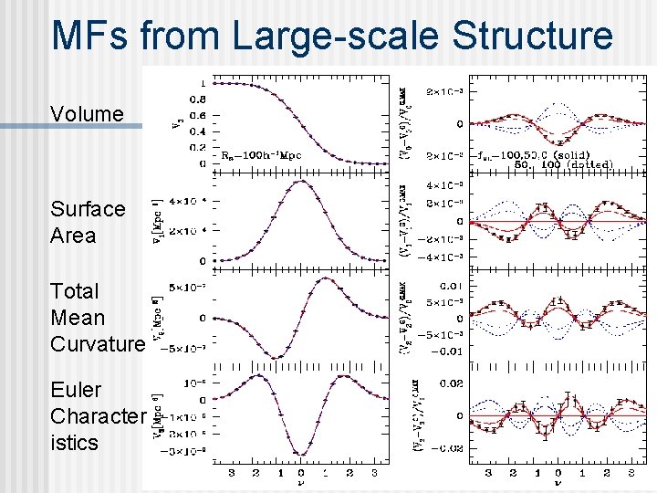
Large-scale Structure Skewness Parameters n n Primordial signal dominates only at a few hundred Mpc and beyond. Need a large survey volume.

MFs from Large-scale Structure Volume Surface Area Total Mean Curvature Euler Character istics

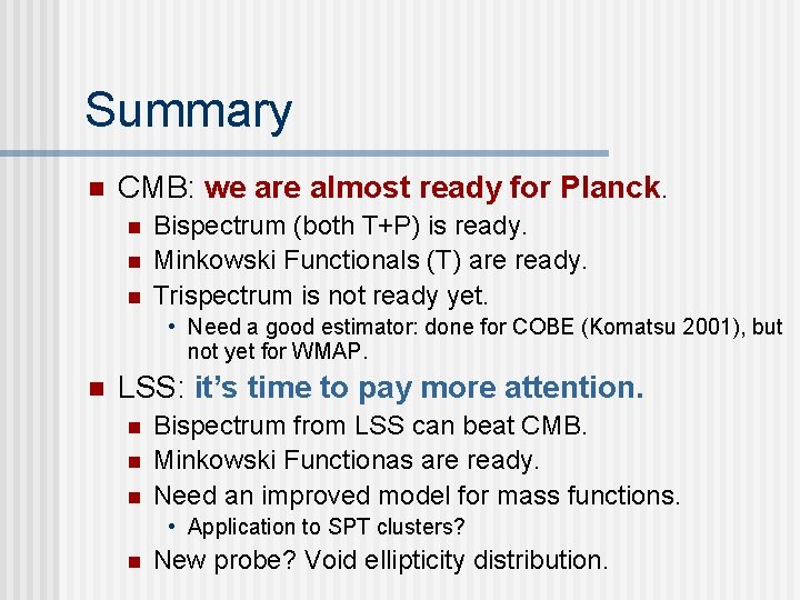
Summary n CMB: we are almost ready for Planck. n n n Bispectrum (both T+P) is ready. Minkowski Functionals (T) are ready. Trispectrum is not ready yet. • Need a good estimator: done for COBE (Komatsu 2001), but not yet for WMAP. n LSS: it’s time to pay more attention. n n n Bispectrum from LSS can beat CMB. Minkowski Functionas are ready. Need an improved model for mass functions. • Application to SPT clusters? n New probe? Void ellipticity distribution.