Estimation We Dont Know Anything For Sure PMFs

Estimation

We Don’t Know Anything For Sure • PMFs and PDFs tell us about what to expect from data when we measure it, including how “uncertain” we are about our measurements but… • PMFs and PDFs depend on parameters that we don’t know. • All we really have is data… • We can’t make much use of PMFs or PDFs without values for their parameters, so what can we do? ? Learn to read crystal balls? ? The Telegraph 2009

We Don’t Know Anything For Sure • In the absence of having a functioning crystal ball, we can take two routes: • Assume the parameters are actual numbers that are fixed and exist, we just don’t know them • Leverage data we can actually measure to infer what their values may be as “best” we can • This is called frequentist inference, and comprises the most common approach. • Assume the parameters r. v. s just like data. • Assume a “prior” dist. which represents your “beliefs” about the parameters before you’ve seen data. Combine that with data to get “updated beliefs” about the parameters. • This is called Bayesian inference, and is generally much more difficult to carry out.

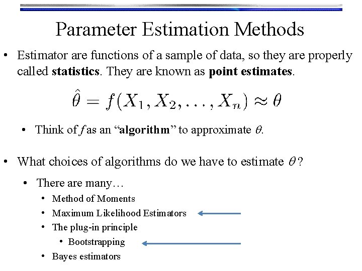
Parameter Estimation Methods • Estimator are functions of a sample of data, so they are properly called statistics. They are known as point estimates. • Think of f as an “algorithm” to approximate q. • What choices of algorithms do we have to estimate q ? • There are many… • Method of Moments • Maximum Likelihood Estimators • The plug-in principle • Bootstrapping • Bayes estimators

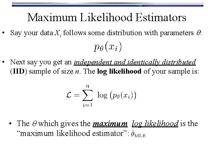
Maximum Likelihood Estimators • Say your data Xi follows some distribution with parameters q: • Next say you get an independent and identically distributed (IID) sample of size n. The log likelihood of your sample is: • The q which gives the maximum log likelihood is the “maximum likelihood estimator”:

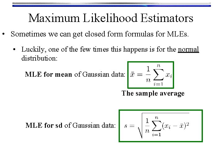
Maximum Likelihood Estimators • Sometimes we can get closed formulas for MLEs. • Luckily, one of the few times this happens is for the normal distribution: MLE for mean of Gaussian data: The sample average MLE for sd of Gaussian data:

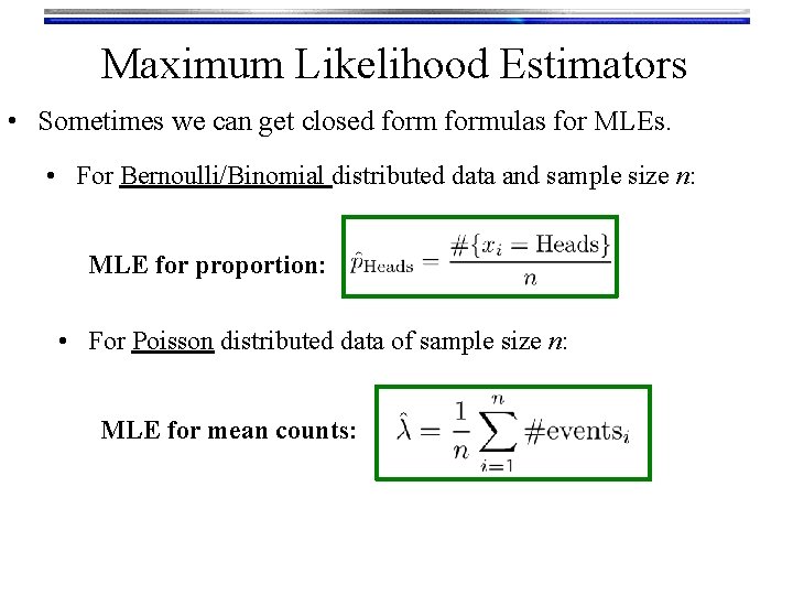
Maximum Likelihood Estimators • Sometimes we can get closed formulas for MLEs. • For Bernoulli/Binomial distributed data and sample size n: MLE for proportion: • For Poisson distributed data of sample size n: MLE for mean counts:

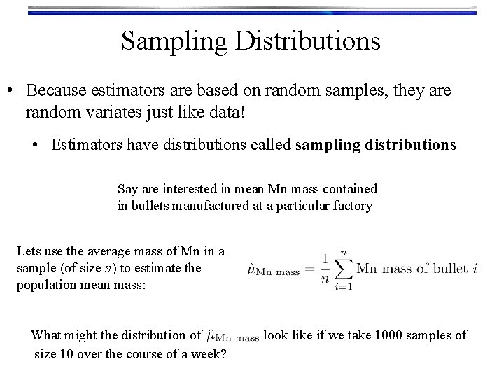
Sampling Distributions • Because estimators are based on random samples, they are random variates just like data! • Estimators have distributions called sampling distributions Say are interested in mean Mn mass contained in bullets manufactured at a particular factory Lets use the average mass of Mn in a sample (of size n) to estimate the population mean mass: What might the distribution of size 10 over the course of a week? look like if we take 1000 samples of

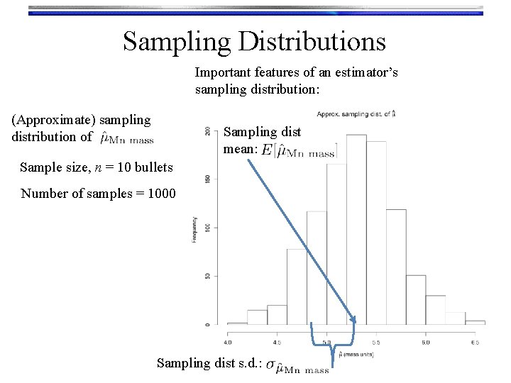
Sampling Distributions Important features of an estimator’s sampling distribution: (Approximate) sampling distribution of Sampling dist mean: Sample size, n = 10 bullets Number of samples = 1000 Sampling dist s. d. :

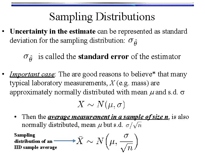
Sampling Distributions • Uncertainty in the estimate can be represented as standard deviation for the sampling distribution: is called the standard error of the estimator • Important case: The are good reasons to believe* that many typical laboratory measurements, X (e. g. mass) are approximately normally distributed with mean m and s. d. s • Then the average measurement in a sample of size n, is also normally distributed, mean m but s. d. Sampling distribution of an IID sample average

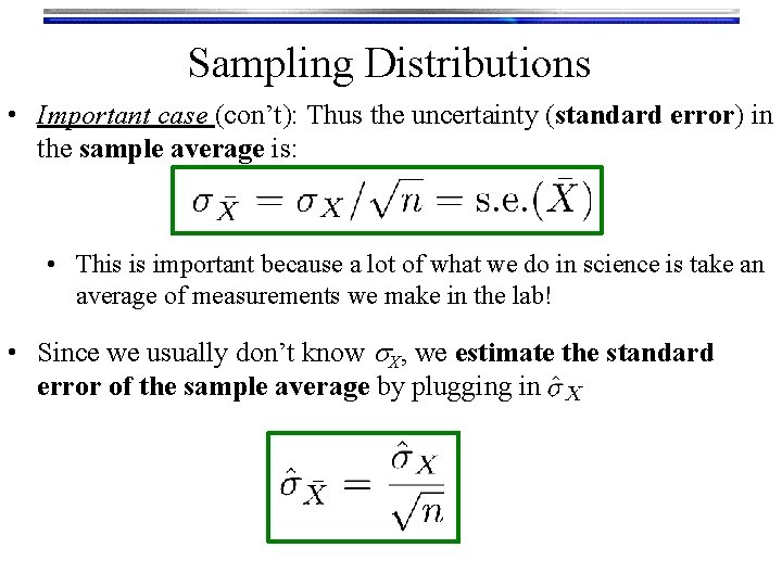
Sampling Distributions • Important case (con’t): Thus the uncertainty (standard error) in the sample average is: • This is important because a lot of what we do in science is take an average of measurements we make in the lab! • Since we usually don’t know s. X, we estimate the standard error of the sample average by plugging in

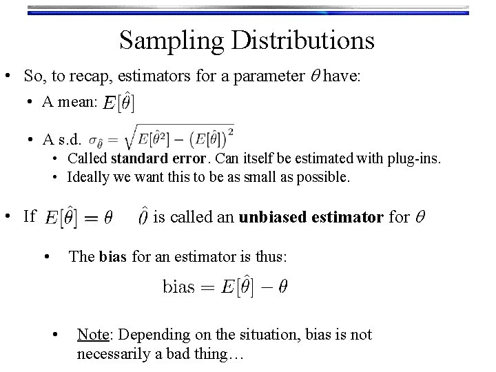
Sampling Distributions • So, to recap, estimators for a parameter q have: • A mean: • A s. d. • Called standard error. Can itself be estimated with plug-ins. • Ideally we want this to be as small as possible. is called an unbiased estimator for q • If • The bias for an estimator is thus: • Note: Depending on the situation, bias is not necessarily a bad thing…

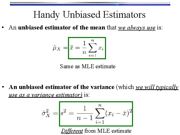
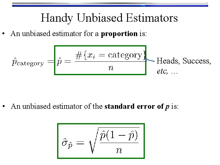
Handy Unbiased Estimators • An unbiased estimator of the mean that we always use is: Same as MLE estimate • An unbiased estimator of the variance (which we will typically use as a variance estimator) is: Different from MLE estimate

Handy Unbiased Estimators • An unbiased estimator for a proportion is: Heads, Success, etc, … • An unbiased estimator of the standard error of p is:

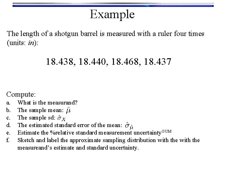
Example The length of a shotgun barrel is measured with a ruler four times (units: in): 18. 438, 18. 440, 18. 468, 18. 437 Compute: a. b. c. d. e. f. What is the measurand? The sample mean: The sample sd: The estimated standard error of the mean: Estimate the %relative standard measurement uncertainty. GUM Sketch and label the approximate sampling distribution with the measureand’s estimate and standard uncertainty.

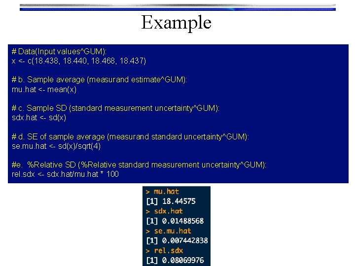
Example # Data(Input values^GUM): x <- c(18. 438, 18. 440, 18. 468, 18. 437) # b. Sample average (measurand estimate^GUM): mu. hat <- mean(x) # c. Sample SD (standard measurement uncertainty^GUM): sdx. hat <- sd(x) # d. SE of sample average (measurand standard uncertainty^GUM): se. mu. hat <- sd(x)/sqrt(4) #e. %Relative SD (%Relative standard measurement uncertainty^GUM): rel. sdx <- sdx. hat/mu. hat * 100

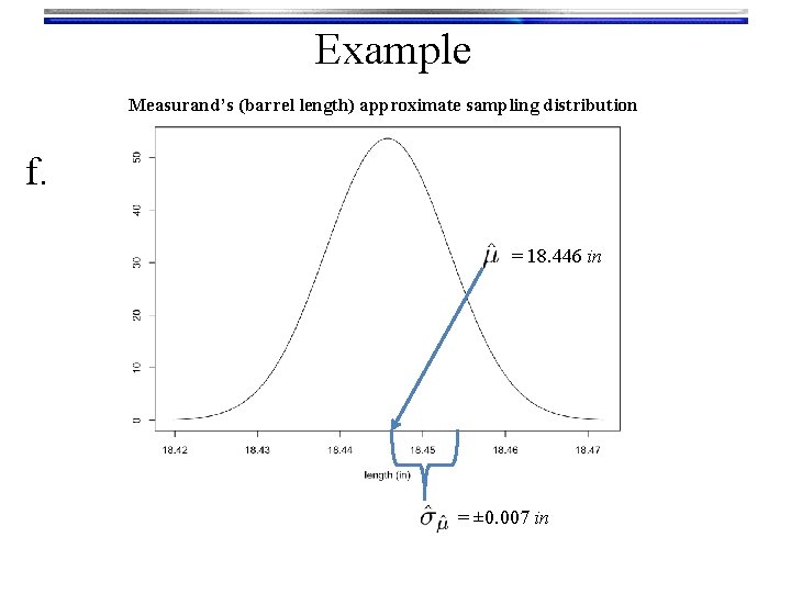
Example Measurand’s (barrel length) approximate sampling distribution f. = 18. 446 in = ± 0. 007 in

The Bootstrap • Reality in lab work: • Sample sizes are often small • Parameters we may want estimates for don’t have a known or convenient sampling distribution • Reality in the 21 st century: • Computers are powerful, cheap and plentiful! • The bootstrap is a computer based simulation method that can be used to estimate virtually any parameter along with a measure of its accuracy. Efron • Assumes nothing about the underlying data except that it is IID • Tends to give good estimates even for small sample sizes Both handy properties forensic applications

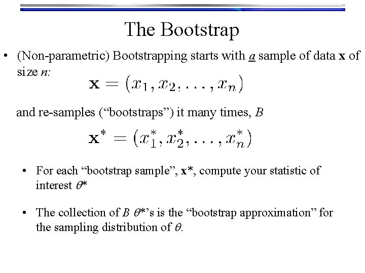
The Bootstrap • (Non-parametric) Bootstrapping starts with a sample of data x of size n: and re-samples (“bootstraps”) it many times, B • For each “bootstrap sample”, x*, compute your statistic of interest q* • The collection of B q*’s is the “bootstrap approximation” for the sampling distribution of q.

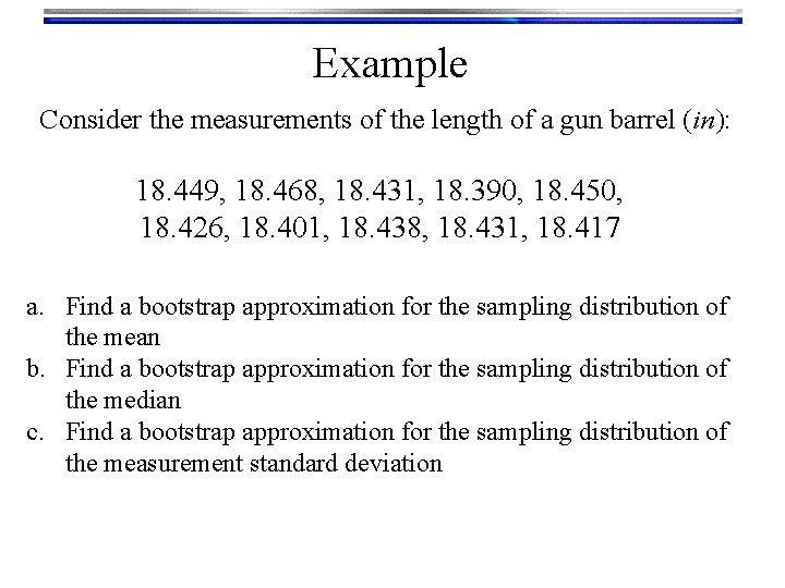
Example Consider the measurements of the length of a gun barrel (in): 18. 449, 18. 468, 18. 431, 18. 390, 18. 450, 18. 426, 18. 401, 18. 438, 18. 431, 18. 417 a. Find a bootstrap approximation for the sampling distribution of the mean b. Find a bootstrap approximation for the sampling distribution of the median c. Find a bootstrap approximation for the sampling distribution of the measurement standard deviation

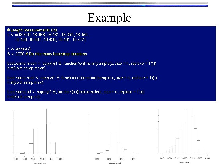
Example # Length measurements (in): x <- c(18. 449, 18. 468, 18. 431, 18. 390, 18. 450, 18. 426, 18. 401, 18. 438, 18. 431, 18. 417) n <- length(x) B <- 2000 # Do this many bootstrap iterations boot. samp. mean <- sapply(1: B, function(xx){mean(sample(x, size = n, replace = T))}) hist(boot. samp. mean) boot. samp. med <- sapply(1: B, function(xx){median(sample(x, size = n, replace = T))}) hist(boot. samp. med) boot. samp. sd <- sapply(1: B, function(xx){sd(sample(x, size = n, replace = T))}) hist(boot. samp. sd)

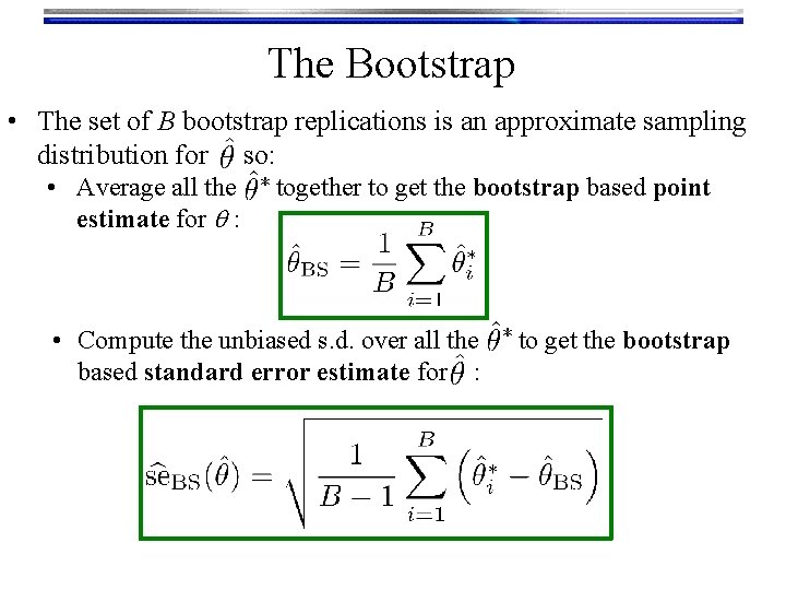
The Bootstrap • The set of B bootstrap replications is an approximate sampling distribution for so: • Average all the together to get the bootstrap based point estimate for q : • Compute the unbiased s. d. over all the to get the bootstrap based standard error estimate for :

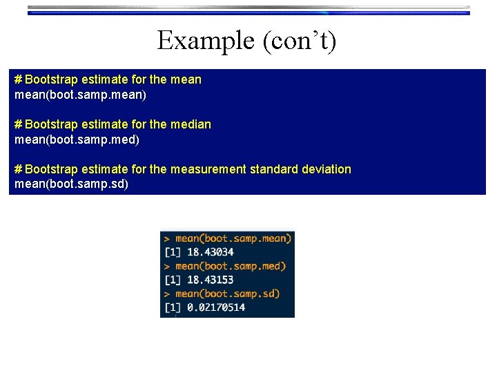
Example (con’t) # Bootstrap estimate for the mean(boot. samp. mean) # Bootstrap estimate for the median mean(boot. samp. med) # Bootstrap estimate for the measurement standard deviation mean(boot. samp. sd)

Example: Bootstrapping Fail How would our last bootstrap algorithm be different for estimating the standard error of a sample max over a uniform distribution? We will simulate some fake data from a uniform distribution with known min = 1 and known max = 3. The sample size will be n = 15. 1. 891304, 2. 909405, 1. 417487, 1. 386373, 1. 070313, 1. 031299, 2. 010315, 2. 537558, 1. 424424, 2. 286100, 1. 385528, 1. 608154, 1. 102906, 2. 753568, 1. 010469

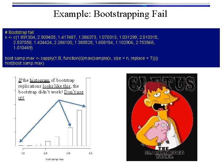
Example: Bootstrapping Fail # Bootstrap fail: x <- c(1. 891304, 2. 909405, 1. 417487, 1. 386373, 1. 070313, 1. 031299, 2. 010315, 2. 537558, 1. 424424, 2. 286100, 1. 385528, 1. 608154, 1. 102906, 2. 753568, 1. 010469) boot. samp. max <- sapply(1: B, function(i){max(sample(x, size = n, replace = T))}) hist(boot. samp. max) If the histogram of bootstrap replications looks like this, the bootstrap didn’t work! Don’t use it!!

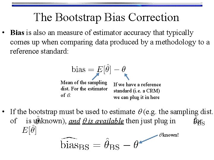
The Bootstrap Bias Correction • Bias is also an measure of estimator accuracy that typically comes up when comparing data produced by a methodology to a reference standard: Mean of the sampling If we have a reference dist. For the estimator standard (i. e. a CRM) of q. we can plug it in here • If the bootstrap must be used to estimate q (e. g. the sampling dist. of is unknown), and q is available then just plug in for q known!

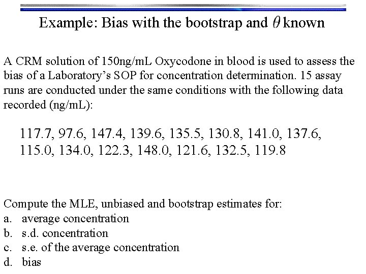
Example: Bias with the bootstrap and known A CRM solution of 150 ng/m. L Oxycodone in blood is used to assess the bias of a Laboratory’s SOP for concentration determination. 15 assay runs are conducted under the same conditions with the following data recorded (ng/m. L): 117. 7, 97. 6, 147. 4, 139. 6, 135. 5, 130. 8, 141. 0, 137. 6, 115. 0, 134. 0, 122. 3, 148. 0, 121. 6, 132. 5, 119. 8 Compute the MLE, unbiased and bootstrap estimates for: a. average concentration b. s. d. concentration c. s. e. of the average concentration d. bias

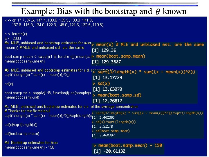
Example: Bias with the bootstrap and known x <- c(117. 7, 97. 6, 147. 4, 139. 6, 135. 5, 130. 8, 141. 0, 137. 6, 115. 0, 134. 0, 122. 3, 148. 0, 121. 6, 132. 5, 119. 8) n <- length(x) B <- 2000 #a. MLE, unbiased and bootstrap estimates for average concentration mean(x) # MLE and unbiased est. are the same boot. samp. mean <- sapply(1: B, function(i){mean(sample(x, size = n, replace = T))}) mean(boot. samp. mean) #b. MLE, unbiased and bootstrap estimates for s. d. concentration sqrt(1/length(x) * sum((x - mean(x))^2)) sd(x) boot. samp. sd <- sapply(1: B, function(i){sd(sample(x, size = n, replace = T))}) mean(boot. samp. sd) #c. MLE, unbiased and bootstrap estimates for s. e. of the average concentration # Thanks for the fix Helen. J! sqrt(1/length(x) * sum((x - mean(x))^2))/sqrt(length(x)) sd(x)/sqrt(length(x)) sd(boot. samp. mean) #d. Bootstrap estimates for bias mean(boot. samp. mean) - 150