Estimation and Confidence Intervals Chapter Nine Mc GrawHillIrwin

Estimation and Confidence Intervals Chapter Nine Mc. Graw-Hill/Irwin © 2006 The Mc. Graw-Hill Companies, Inc. , All Rights Reserved.

A Point estimate is a single value (statistic) used to estimate a population value (parameter). Eg. μx is a point estimate of μ We cannot be sure that Point estimate is the mean. But we can calculate an interval around this estimate and assert with a certain confidence that the true population mean will lie inside it. A Confidence Interval is a range of values within which the population parameter (eg. μ ) is expected to occur at a specified level of confidence generally expressed as a percent.

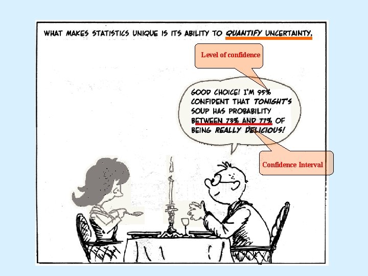
Level of confidence Confidence Interval

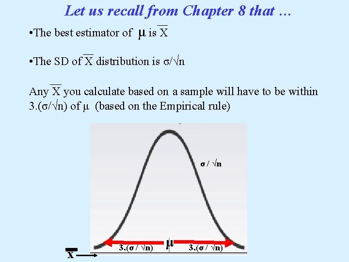
Let us recall from Chapter 8 that … • The best estimator of μ is X • The SD of X distribution is σ/√n Any X you calculate based on a sample will have to be within 3. (σ/√n) of μ (based on the Empirical rule) σ/√n σ / √n x 3. (σ / √n) μ 3. (σ / √n)

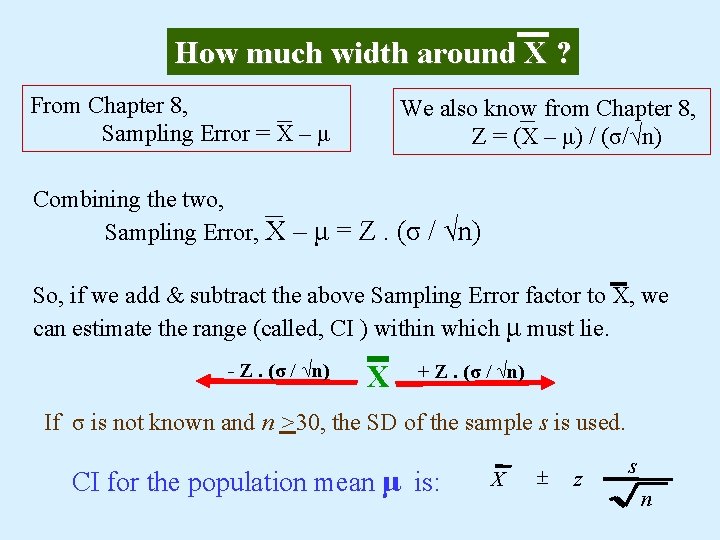
How much width around X ? From Chapter 8, Sampling Error = X – μ We also know from Chapter 8, Z = (X – μ) / (σ/√n) Combining the two, Sampling Error, X – μ = Z. (σ / √n) So, if we add & subtract the above Sampling Error factor to X, we can estimate the range (called, CI ) within which μ must lie. - Z. (σ / √n) X + Z. (σ / √n) If σ is not known and n >30, the SD of the sample s is used. CI for the population mean μ is: X ± z s n

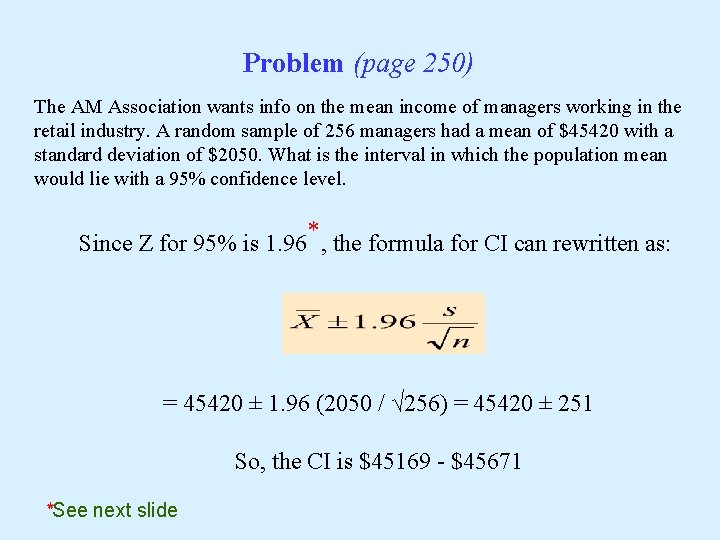
Problem (page 250) The AM Association wants info on the mean income of managers working in the retail industry. A random sample of 256 managers had a mean of $45420 with a standard deviation of $2050. What is the interval in which the population mean would lie with a 95% confidence level. Since Z for 95% is 1. 96*, the formula for CI can rewritten as: = 45420 ± 1. 96 (2050 / √ 256) = 45420 ± 251 So, the CI is $45169 - $45671 *See next slide

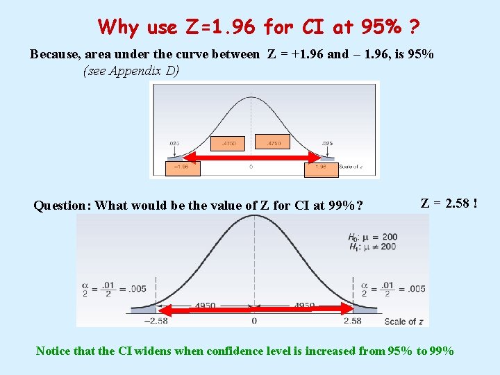
Why use Z=1. 96 for CI at 95% ? Because, area under the curve between Z = +1. 96 and – 1. 96, is 95% (see Appendix D) Question: What would be the value of Z for CI at 99%? Z = 2. 58 ! Notice that the CI widens when confidence level is increased from 95% to 99%

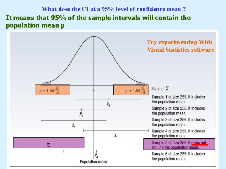
What does the CI at a 95% level of confidence mean ? It means that 95% of the sample intervals will contain the population mean μ Try experimenting With Visual Statistics software

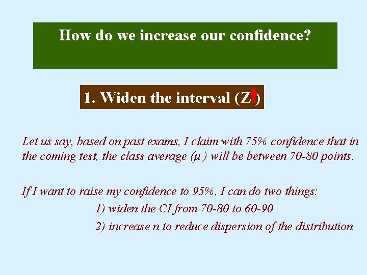
How do we increase our confidence? 1. Widen the interval (Z ) Let us say, based on past exams, I claim with 75% confidence that in the coming test, the class average (μ ) will be between 70 -80 points. If I want to raise my confidence to 95%, I can do two things: 1) widen the CI from 70 -80 to 60 -90 2) increase n to reduce dispersion of the distribution

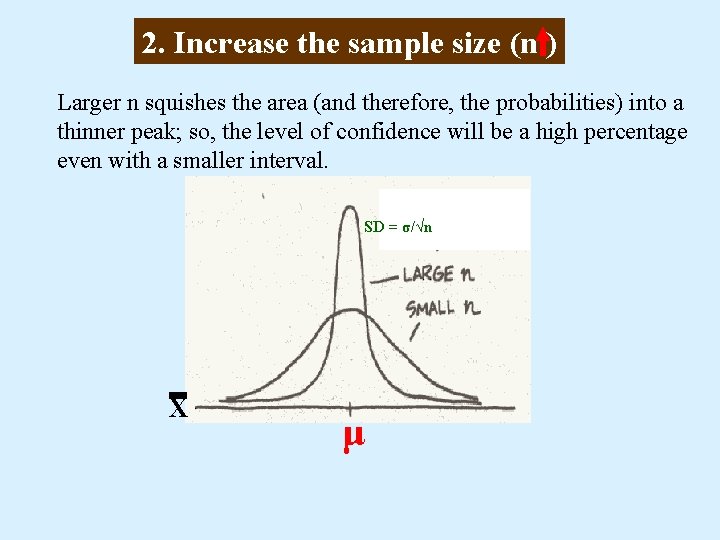
2. Increase the sample size (n ) Larger n squishes the area (and therefore, the probabilities) into a thinner peak; so, the level of confidence will be a high percentage even with a smaller interval. SD = σ/√n X μ

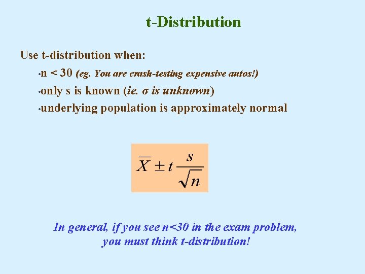
t-Distribution Use t-distribution when: • n < 30 (eg. You are crash-testing expensive autos!) • only s is known (ie. σ is unknown) • underlying population is approximately normal In general, if you see n<30 in the exam problem, you must think t-distribution!

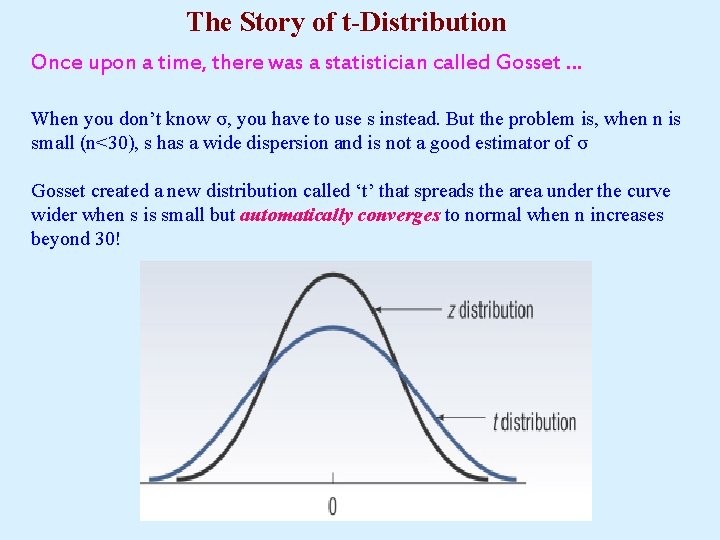
The Story of t-Distribution Once upon a time, there was a statistician called Gosset … When you don’t know σ, you have to use s instead. But the problem is, when n is small (n<30), s has a wide dispersion and is not a good estimator of σ Gosset created a new distribution called ‘t’ that spreads the area under the curve wider when s is small but automatically converges to normal when n increases beyond 30!

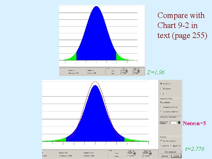
Compare with Chart 9 -2 in text (page 255) Z=1. 96 Note: n=5 t=2. 776

Visual Statistics Demo Using Continuous Distribution module

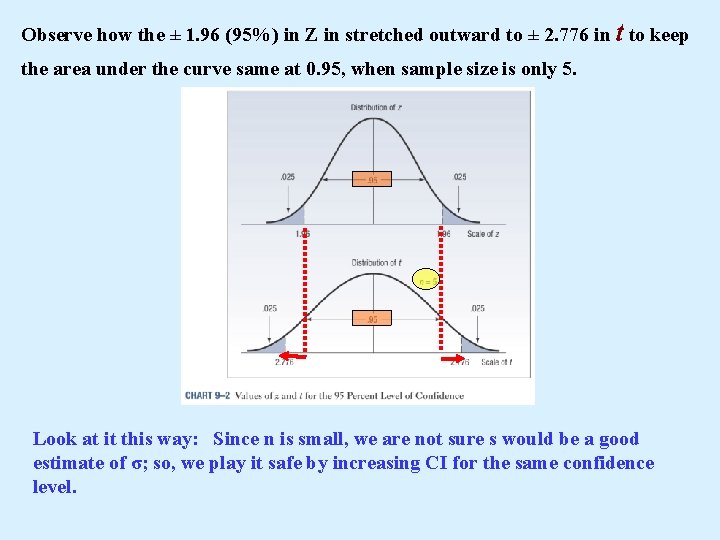
Observe how the ± 1. 96 (95%) in Z in stretched outward to ± 2. 776 in t to keep the area under the curve same at 0. 95, when sample size is only 5. Look at it this way: Since n is small, we are not sure s would be a good estimate of σ; so, we play it safe by increasing CI for the same confidence level.

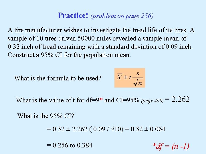
Practice! (problem on page 256) A tire manufacturer wishes to investigate the tread life of its tires. A sample of 10 tires driven 50000 miles revealed a sample mean of 0. 32 inch of tread remaining with a standard deviation of 0. 09 inch. Construct a 95% CI for the population mean. What is the formula to be used? What is the value of t for df=9* and CI=95% (page 498) = 2. 262 What is the 95% CI? = 0. 32 ± 2. 262 ( 0. 09 / √ 10) = 0. 32 ± 0. 064 = 0. 256 to 0. 384 *df = (n -1)

Degrees of Freedom You are in a room with 10 chairs and you are sitting in one of them. The other chairs are empty. How many other chairs can you move to? Ans: 9 So in general, df = n-1

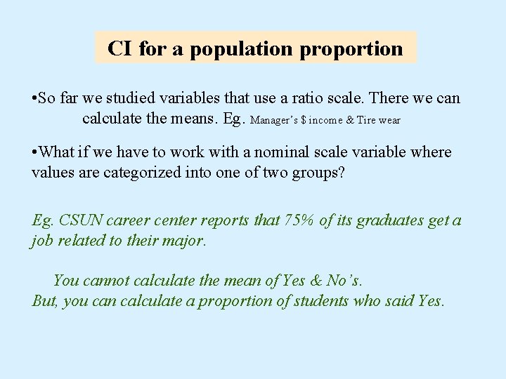
CI for a population proportion • So far we studied variables that use a ratio scale. There we can calculate the means. Eg. Manager’s $ income & Tire wear • What if we have to work with a nominal scale variable where values are categorized into one of two groups? Eg. CSUN career center reports that 75% of its graduates get a job related to their major. You cannot calculate the mean of Yes & No’s. But, you can calculate a proportion of students who said Yes.

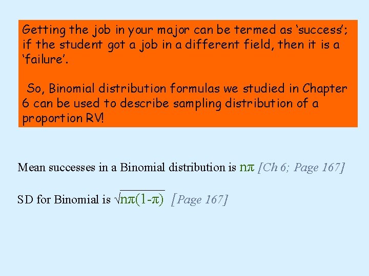
Getting the job in your major can be termed as ‘success’; if the student got a job in a different field, then it is a ‘failure’. So, Binomial distribution formulas we studied in Chapter 6 can be used to describe sampling distribution of a proportion RV! Mean successes in a Binomial distribution is nπ [Ch 6; Page 167] SD for Binomial is √nπ(1 -π) [Page 167]

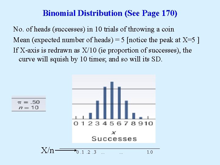
Binomial Distribution (See Page 170) No. of heads (successes) in 10 trials of throwing a coin Mean (expected number of heads) = 5 [notice the peak at X=5 ] If X-axis is redrawn as X/10 (ie proportion of successes), the curve will squish by 10 times; and so will its SD. X/n 0. 1. 2. 3 . . . 1. 0

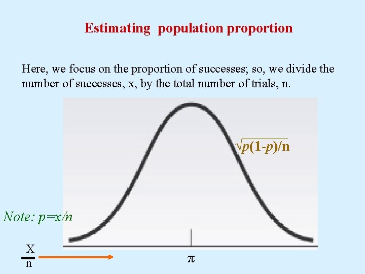
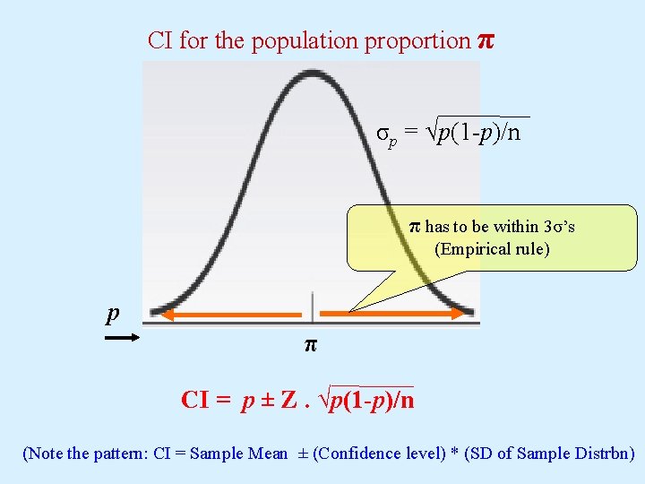
Estimating population proportion Here, we focus on the proportion of successes; so, we divide the number of successes, x, by the total number of trials, n. √p(1 -p)/n Note: p=x/n X n π

CI for the population proportion π σp = √p(1 -p)/n π has to be within 3σ’s (Empirical rule) p π CI = p ± Z. √p(1 -p)/n (Note the pattern: CI = Sample Mean ± (Confidence level) * (SD of Sample Distrbn)

A sample of 500 executives who own their own home revealed 175 planned to sell their homes and retire to Arizona. Develop a 98% confidence interval for the proportion of executives that plan to sell and move to Arizona.

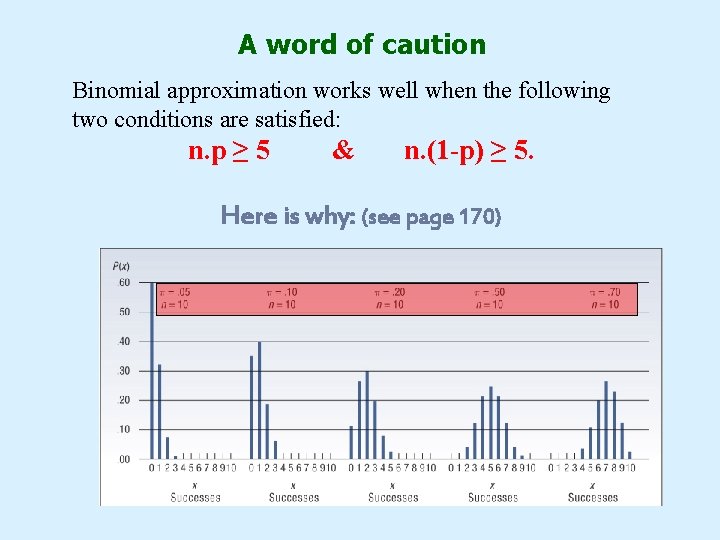
A word of caution Binomial approximation works well when the following two conditions are satisfied: n. p ≥ 5 & n. (1 -p) ≥ 5. Here is why: (see page 170)

Calculating the sample size 3 factors affect the sample size: • The level of confidence desired • The margin of error the researcher will tolerate. • The variability in the population being studied.

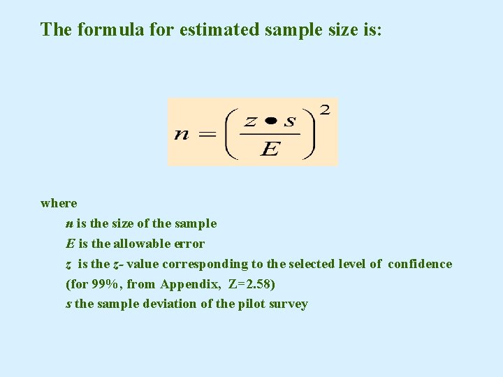
The formula for estimated sample size is: where n is the size of the sample E is the allowable error z is the z- value corresponding to the selected level of confidence (for 99%, from Appendix, Z=2. 58) s the sample deviation of the pilot survey

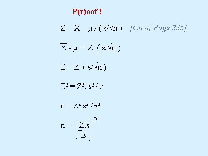
P(r)oof ! Z = X – μ / ( s/√n ) [Ch 8; Page 235] X - μ = Z. ( s/√n ) E 2 = Z 2. s 2 / n n = Z 2. s 2 /E 2 n = Z. s E 2

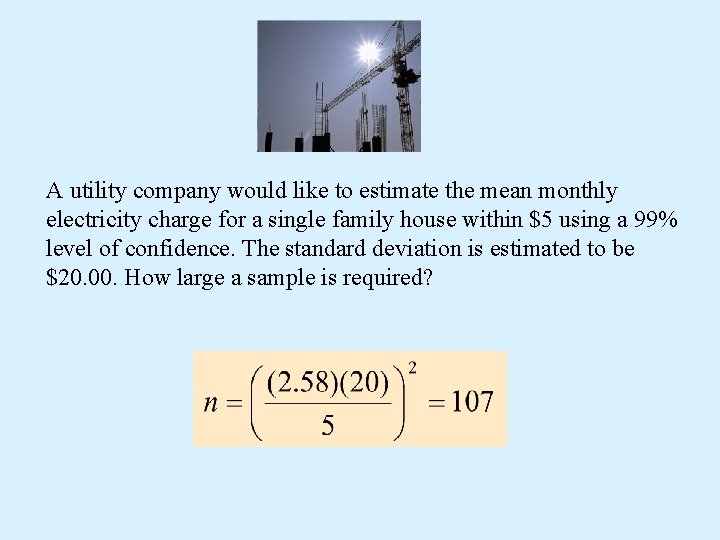
A utility company would like to estimate the mean monthly electricity charge for a single family house within $5 using a 99% level of confidence. The standard deviation is estimated to be $20. 00. How large a sample is required?

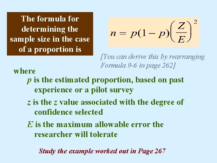
The formula for determining the sample size in the case of a proportion is [You can derive this by rearranging Formula 9 -6 in page 262] where p is the estimated proportion, based on past experience or a pilot survey z is the z value associated with the degree of confidence selected E is the maximum allowable error the researcher will tolerate Study the example worked out in Page 267

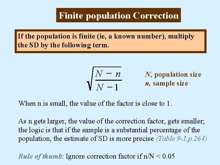
Finite population Correction If the population is finite (ie, a known number), multiply the SD by the following term. N - n N -1 N, population size n, sample size When n is small, the value of the factor is close to 1. As n gets larger, the value of the correction factor, gets smaller; the logic is that if the sample is a substantial percentage of the population, the estimate of SD is more precise (Table 9 -1, p. 264) Rule of thumb: Ignore correction factor if n/N < 0. 05