Environmental Data Analysis with Mat Lab Lecture 20

Environmental Data Analysis with Mat. Lab Lecture 20: Coherence; Tapering and Spectral Analysis

SYLLABUS Lecture 01 Lecture 02 Lecture 03 Lecture 04 Lecture 05 Lecture 06 Lecture 07 Lecture 08 Lecture 09 Lecture 10 Lecture 11 Lecture 12 Lecture 13 Lecture 14 Lecture 15 Lecture 16 Lecture 17 Lecture 18 Lecture 19 Lecture 20 Lecture 21 Lecture 22 Lecture 23 Lecture 24 Using Mat. Lab Looking At Data Probability and Measurement Error Multivariate Distributions Linear Models The Principle of Least Squares Prior Information Solving Generalized Least Squares Problems Fourier Series Complex Fourier Series Lessons Learned from the Fourier Transform Power Spectral Density Filter Theory Applications of Filters Factor Analysis Orthogonal functions Covariance and Autocorrelation Cross-correlation Smoothing, Correlation and Spectra Coherence; Tapering and Spectral Analysis Interpolation Hypothesis testing Hypothesis Testing continued; F-Tests Confidence Limits of Spectra, Bootstraps

purpose of the lecture Part 1 Finish up the discussion of correlations between time series Part 2 Examine how the finite observation time affects estimates of the power spectral density of time series

Part 1 “Coherence” frequency-dependent correlations between time series

Scenario A in a hypothetical region windiness and temperature correlate at periods of a year, because of large scale climate patterns but they do not correlate at periods of a few days

wind speed 1 2 3 temperature time, years 1 2 time, years 3

summer hot and windy wind speed winters cool and calm 1 2 3 temperature time, years 1 2 time, years 3

wind speed heat wave not especially windy 1 cold snap not especially calm 2 3 temperature time, years 1 2 time, years 3

in this case times series correlated at long periods but not at short periods

Scenario B in a hypothetical region plankton growth rate and precipitation correlate at periods of a few weeks but they do not correlate seasonally

growth rate 1 2 3 precipitation time, years 1 2 time, years 3

plant growth rate has no seasonal signal 1 summer drier than winter 2 3 precipitation time, years 1 2 time, years 3

plant growth rate high at times of peak precipitation 1 2 3 precipitation time, years 1 2 time, years 3

in this case times series correlated at short periods but not at long periods

Coherence a way to quantify frequency-dependent correlation
 and v(t) around frequency, ω0")
strategy band pass filter the two time series, u(t) and v(t) around frequency, ω0 compute their zero-lag cross correlation (large when time series are similar in shape) repeat for many ω0’s to create a function c(ω0)
 has this p. s. d. 2Δω |f(ω)|2 2Δω ω -ω0")
band pass filter f(t) has this p. s. d. 2Δω |f(ω)|2 2Δω ω -ω0 0 ω0

evaluate at zero lag t=0 and at many ω0’s

Short Cut Fact 1 A function evaluates at time t=0 is equal to the integral of its Fourier Transform Fact 2 the Fourier Transform of a convolution is the product of the transforms
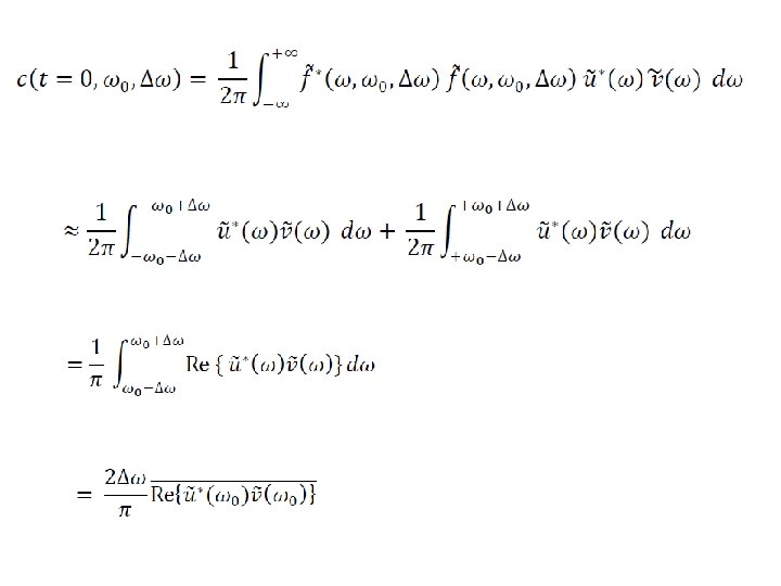

integral over frequency

integral over frequency assume ideal band pass filter that is either 0 or 1 negative frequencies positive frequencies

integral over frequency assume ideal band pass filter that is either 0 or 1 negative frequencies positive frequencies c is real so real part is symmetric, adds imag part is antisymmetric, cancels

integral over frequency assume ideal band pass filter that is either 0 or 1 negative frequencies positive frequencies c is real so real part is symmetric, adds imag part is antisymmetric, cancels interpret intergral as an average over frequency band

integral over frequency can be viewed as an average over frequency (indicated with the overbar)
 2.")
Two final steps 1. Omit taking of real part in formula (simplifying approximation) 2. Normalize by the amplitude of the two time series and square, so that result varies between 0 and 1

the final result is called Coherence
 B) new dataset: C) Water Quality D) Reynolds Channel, Coastal Long Island, New")
A) B) new dataset: C) Water Quality D) Reynolds Channel, Coastal Long Island, New York E) F)
 air temperature B) new dataset: water temperature C) Water Quality D) Reynolds")
precipitation A) air temperature B) new dataset: water temperature C) Water Quality D) Reynolds Channel, Coastal Long Island, New York salinity E) turbidity F) chlorophyl
 periods near 1 year B) periods near 5 days Fig, 9. 18. Band-pass")
A) periods near 1 year B) periods near 5 days Fig, 9. 18. Band-pass filtered water quality measurements from Reynolds Channel (New York) for several years starting January 1, 2006. A) Periods near one year; and B) periods near 5 days. Mat. Lab script eda 09_16.
 A) one year one week C)")
B) A) one year one week C)
 A) C) one year one week")
high coherence at periods of 1 year B) A) C) one year one week moderate coherence at periods of about a month very low coherence at periods of months to a few days

Part 2 windowing time series before computing powerspectral density

scenario: you are studying an indefinitely long phenomenon … but you only observe a short portion of it …

how does the power spectral density of the short piece differ from the p. s. d. of the indefinitely long phenomenon (assuming stationary time series)

We might suspect that the difference will be increasingly significant as the window of observation becomes so short that it includes just a few oscillations of the period of interest.

starting point short piece is the indefinitely long time series multiplied by a window function, W(t)


by the convolution theorem Fourier Transform of short piece is Fourier Transform of indefinitely long time series convolved with Fourier Transform of window function

so Fourier Transform of short piece exactly Fourier Transform of indefinitely long time series when Fourier Transform of window function is a spike

boxcar window function its Fourier Transform
 function sort of spiky but has side")
boxcar window function its Fourier Transform sinc() function sort of spiky but has side lobes
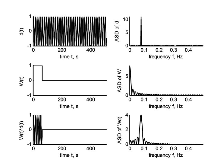

Effect 1: broadening of spectral peaks narrow spectral peak wide central spike wide spectral peak

Effect 2: spurious side lobes only one spectral peak side lobes spurious spectral peaks

Q: Can the situation be improved? A: Yes, by choosing a smoother window function more like a Normal Function (which has no side lobes) but still zero outside of interval of observation

boxcar window function Hamming window function
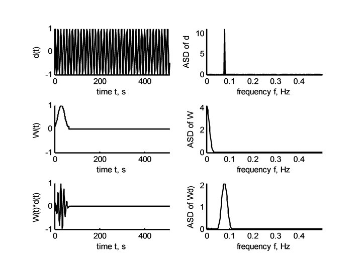

no side lobes but central peak wider than with boxcar

Hamming Window Function

Q: Is there a “best” window function? A: Only if you carefully specify what you mean by “best” (notion of best based on prior information)

“optimal”window function maximize ratio of power in central peak (assumed to lie in range ±ω0 ) to overall power

The parameter, ω0, allows you to choose how much spectral broadening you can tolerate Once ω0 is specified, the problem can be solved by using standard optimization techniques One finds that there actually several window functions, with radically different shapes, that are “optimal”
v Family of three “optimal” window functions v W 2(t)v time, s v")
W 1(t)v Family of three “optimal” window functions v W 2(t)v time, s v W 3(t)v time, s v

a common strategy is to compute the power spectral density with each of these window functions separately and then average the result technique called Multi-taper Spectral Analysis
 time t, s v frequency, Hz v B(t)d(t) v W 1(t)d(t) v v")
d(t) time t, s v frequency, Hz v B(t)d(t) v W 1(t)d(t) v v time t, s v frequency, Hz v W 2(t)d(t) time t, s v frequency, Hz v W 3(t)d(t) time t, s v frequency, Hz v v
 box car tapering time t, s v frequency, Hz v B(t)d(t) frequency, Hz")
d(t) box car tapering time t, s v frequency, Hz v B(t)d(t) frequency, Hz v time t, s v W 1(t)d(t) v v time t, s v frequency, Hz v W 2(t)d(t) time t, s v frequency, Hz v W 3(t)d(t) time t, s v frequency, Hz v v
 v time t, s frequency, Hz v B(t)d(t) Hz time t, s “optimal”")
d(t) v time t, s frequency, Hz v B(t)d(t) Hz time t, s “optimal” tapering with three windowfrequency, functions v v W 1(t)d(t) v v time t, s v frequency, Hz v W 2(t)d(t) time t, s v frequency, Hz v W 3(t)d(t) time t, s v frequency, Hz v v
 time t, s v frequency, Hz v B(t)d(t) v W 1(t)d(t) v v")
d(t) time t, s v frequency, Hz v B(t)d(t) v W 1(t)d(t) v v time t, s v frequency, Hz v W 2(t)d(t) time t, s v frequency, Hz v W 3(t)d(t) time t, s v p. s. d. produced by averaging frequency, Hz v v

Summary always taper a time series before computing the p. s. d. try a simple Hamming taper first it’s simple use multi-taper analysis when higher resolution is needed e. g. when the time series is very short
- Slides: 61