Emissions Uncertainty Inventory and Modeling Framework Case Study

Emissions Uncertainty Inventory and Modeling Framework: Case Study of Residential Wood Combustion Rabab Mashayekhi, Shunliu Zhao, Sahar Saeednooran, Amir Hakami Department of Civil and Environmental Engineering, Carleton University, Ottawa Richard Ménard, Michael Moran, and Junhua Zhang Air Quality Research Division, Environment and Climate Change Canada 1

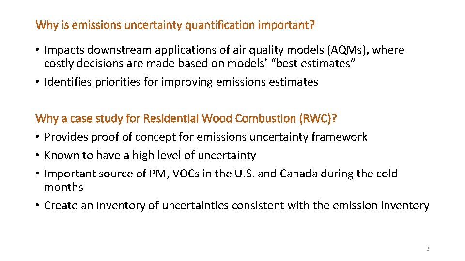
Why is emissions uncertainty quantification important? • Impacts downstream applications of air quality models (AQMs), where costly decisions are made based on models’ “best estimates” • Identifies priorities for improving emissions estimates Why a case study for Residential Wood Combustion (RWC)? • Provides proof of concept for emissions uncertainty framework • Known to have a high level of uncertainty • Important source of PM, VOCs in the U. S. and Canada during the cold months • Create an Inventory of uncertainties consistent with the emission inventory 2

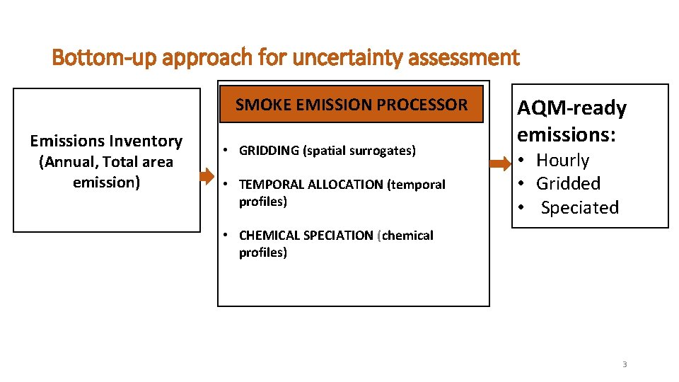
Bottom-up approach for uncertainty assessment SMOKE EMISSION PROCESSOR Emissions Inventory (Annual, Total area emission) • GRIDDING (spatial surrogates) • TEMPORAL ALLOCATION (temporal profiles) AQM-ready emissions: • Hourly • Gridded • Speciated • CHEMICAL SPECIATION (chemical profiles) 3

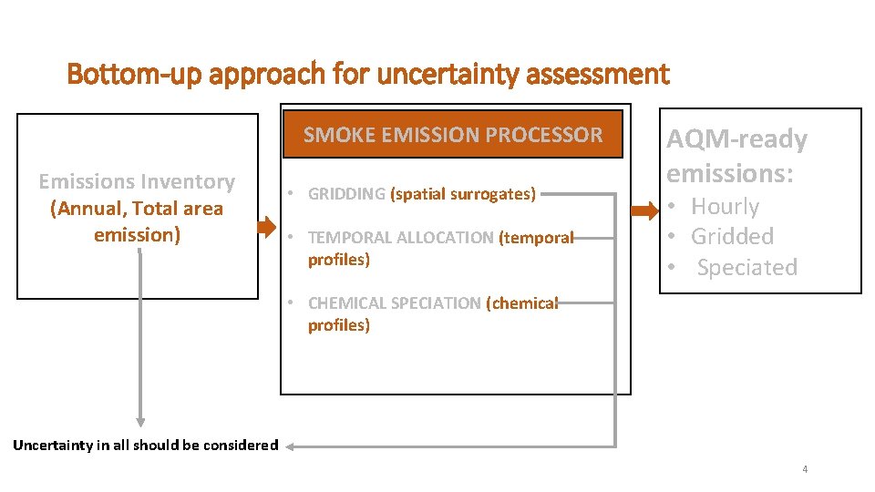
Bottom-up approach for uncertainty assessment SMOKE EMISSION PROCESSOR Emissions Inventory (Annual, Total area emission) • GRIDDING (spatial surrogates) • TEMPORAL ALLOCATION (temporal profiles) AQM-ready emissions: • Hourly • Gridded • Speciated • CHEMICAL SPECIATION (chemical profiles) Uncertainty in all should be considered 4

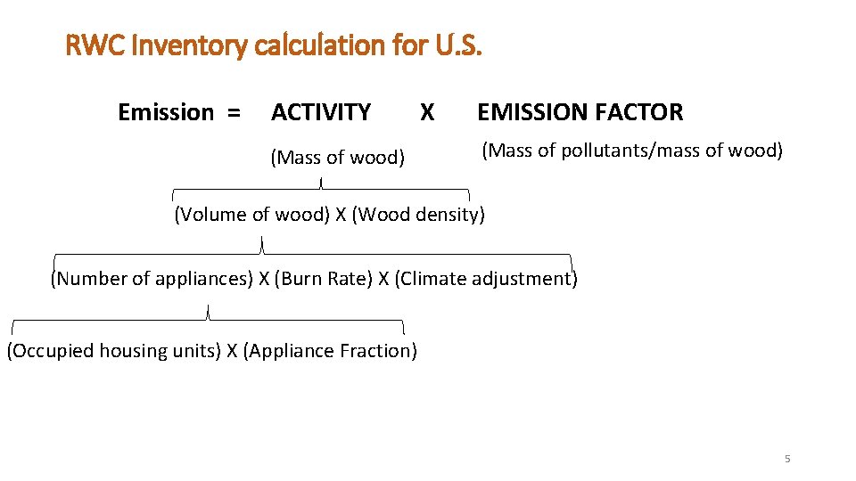
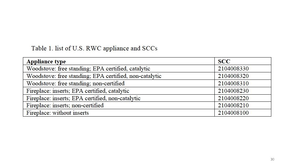
RWC Inventory calculation for U. S. Emission = ACTIVITY (Mass of wood) X EMISSION FACTOR (Mass of pollutants/mass of wood) (Volume of wood) X (Wood density) (Number of appliances) X (Burn Rate) X (Climate adjustment) (Occupied housing units) X (Appliance Fraction) 5

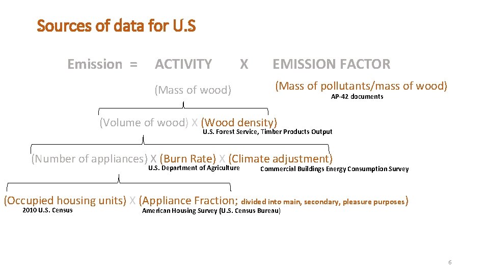
Sources of data for U. S Emission = ACTIVITY (Mass of wood) X EMISSION FACTOR (Mass of pollutants/mass of wood) AP-42 documents (Volume of wood) X (Wood density) U. S. Forest Service, Timber Products Output (Number of appliances) X (Burn Rate) X (Climate adjustment) U. S. Department of Agriculture Commercial Buildings Energy Consumption Survey (Occupied housing units) X (Appliance Fraction; divided into main, secondary, pleasure purposes) 2010 U. S. Census American Housing Survey (U. S. Census Bureau) 6

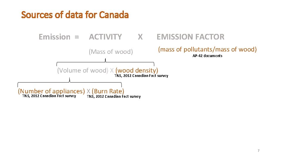
Sources of data for Canada Emission = ACTIVITY X (Mass of wood) EMISSION FACTOR (mass of pollutants/mass of wood) AP-42 documents (Volume of wood) X (wood density) TNS, 2012 Canadian Fact survey (Number of appliances) X (Burn Rate) TNS, 2012 Canadian Fact survey 7

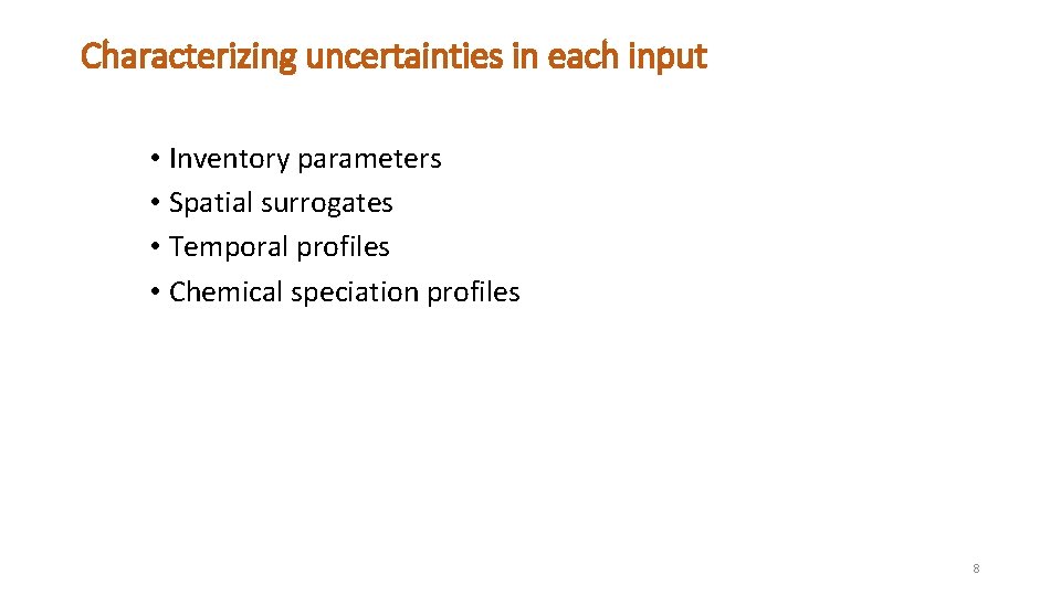
Characterizing uncertainties in each input • Inventory parameters • Spatial surrogates • Temporal profiles • Chemical speciation profiles 8

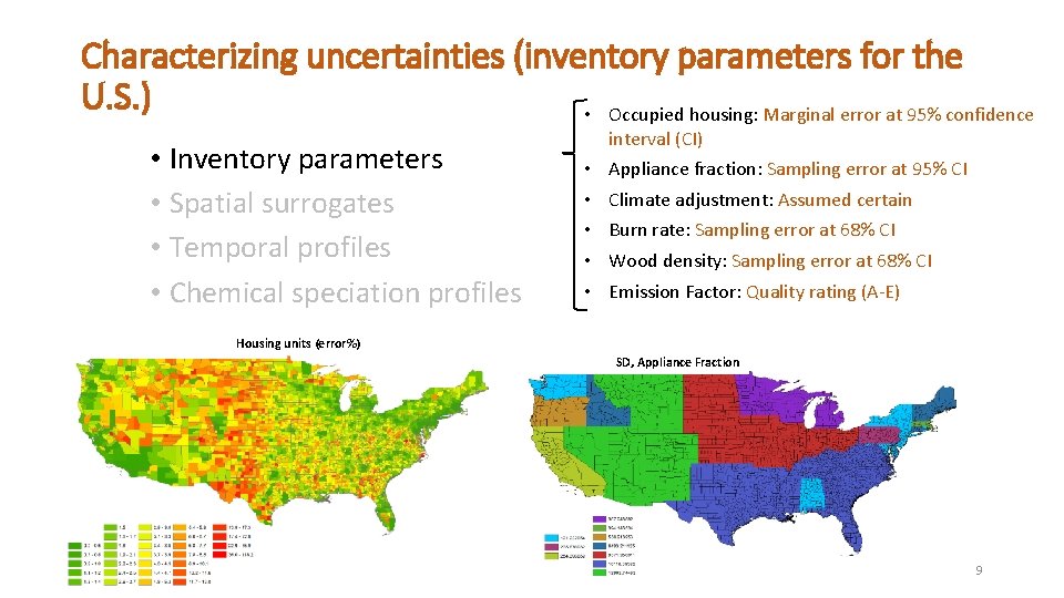
Characterizing uncertainties (inventory parameters for the U. S. ) • Occupied housing: Marginal error at 95% confidence • Inventory parameters • Spatial surrogates • Temporal profiles • Chemical speciation profiles interval (CI) • • • Appliance fraction: Sampling error at 95% CI Climate adjustment: Assumed certain Burn rate: Sampling error at 68% CI Wood density: Sampling error at 68% CI Emission Factor: Quality rating (A-E) Housing units (error%) SD, Appliance Fraction 9

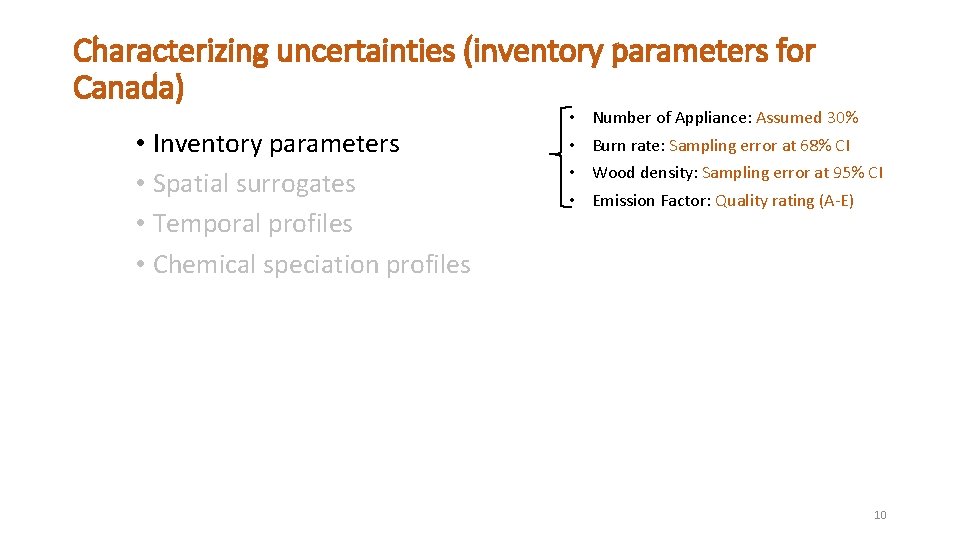
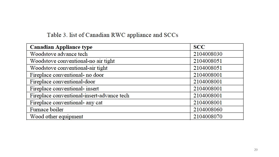
Characterizing uncertainties (inventory parameters for Canada) • Inventory parameters • Spatial surrogates • Temporal profiles • Chemical speciation profiles • • Number of Appliance: Assumed 30% Burn rate: Sampling error at 68% CI Wood density: Sampling error at 95% CI Emission Factor: Quality rating (A-E) 10

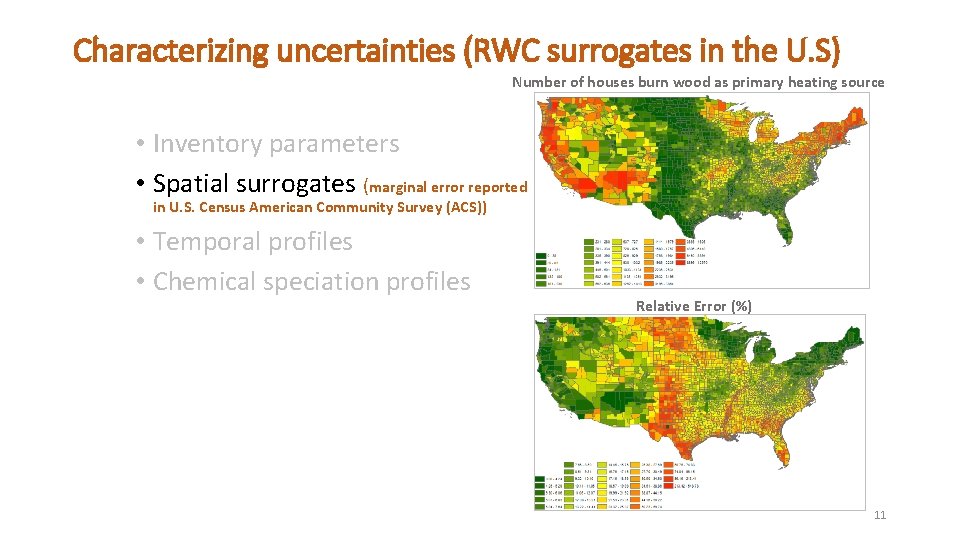
Characterizing uncertainties (RWC surrogates in the U. S) Number of houses burn wood as primary heating source • Inventory parameters • Spatial surrogates (marginal error reported in U. S. Census American Community Survey (ACS)) • Temporal profiles • Chemical speciation profiles Relative Error (%) 11

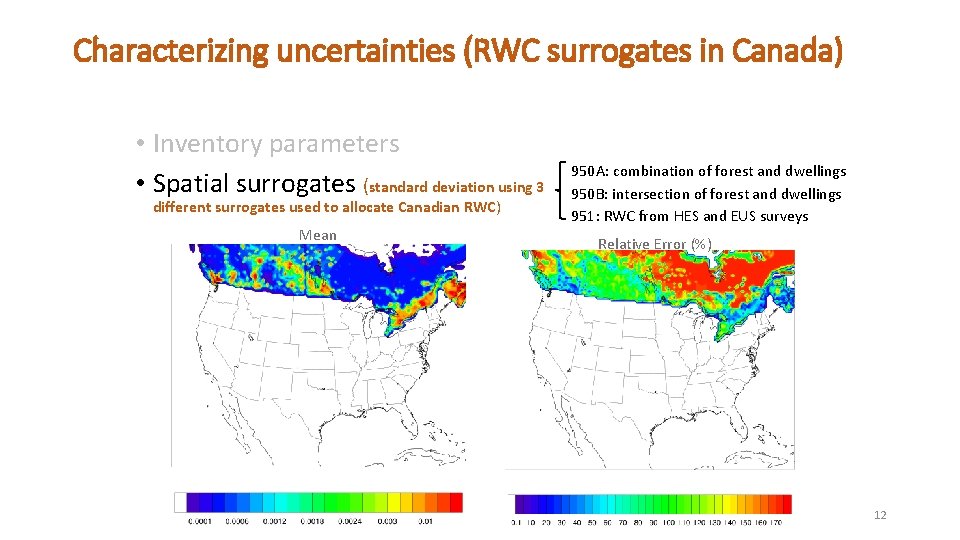
Characterizing uncertainties (RWC surrogates in Canada) • Inventory parameters • Spatial surrogates (standard deviation using 3 different surrogates used to allocate Canadian RWC) Mean 950 A: combination of forest and dwellings 950 B: intersection of forest and dwellings 951: RWC from HES and EUS surveys Relative Error (%) 12

Characterizing uncertainties in each input • Inventory parameters • Surrogates • Temporal profiles • Chemical speciation profiles • We do not have any uncertainties reported in literature • For each temporal and speciation profile, each single coefficient is assigned a standard deviation assuming a 30% uncertainty § Suggestions are welcome! 13

Propagating uncertainties • Monte Carlo simulations • Sampling code is External to SMOKE • Latin Hypercube Sampling (LHS) generates a set of 100 random realizations (other set sizes were also tested) • Normal distribution is assumed for each parameter 14

Results • Resolution: CONUS, 36 km • SMOKE version: v 3. 7 • Episode: February 1 st, 2011 • Chemical speciation: ADOM gas-phase mechanism and 12 -bin aerosol representation (GEM-MACH) 15

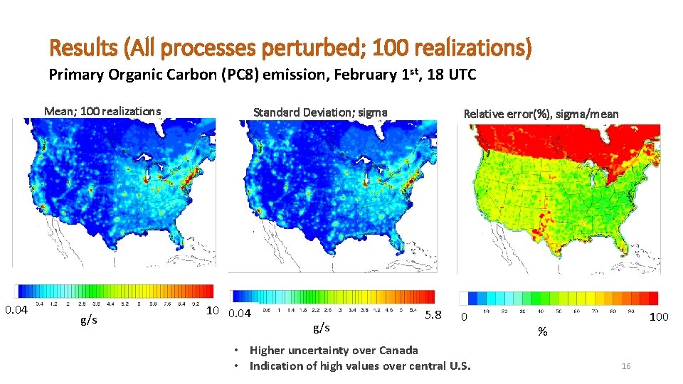
Results (All processes perturbed; 100 realizations) Primary Organic Carbon (PC 8) emission, February 1 st, 18 UTC Mean; 100 realizations 0. 04 g/s Standard Deviation; sigma 10 0. 04 g/s Relative error(%), sigma/mean 5. 8 0 • Higher uncertainty over Canada • Indication of high values over central U. S. 100 % 16

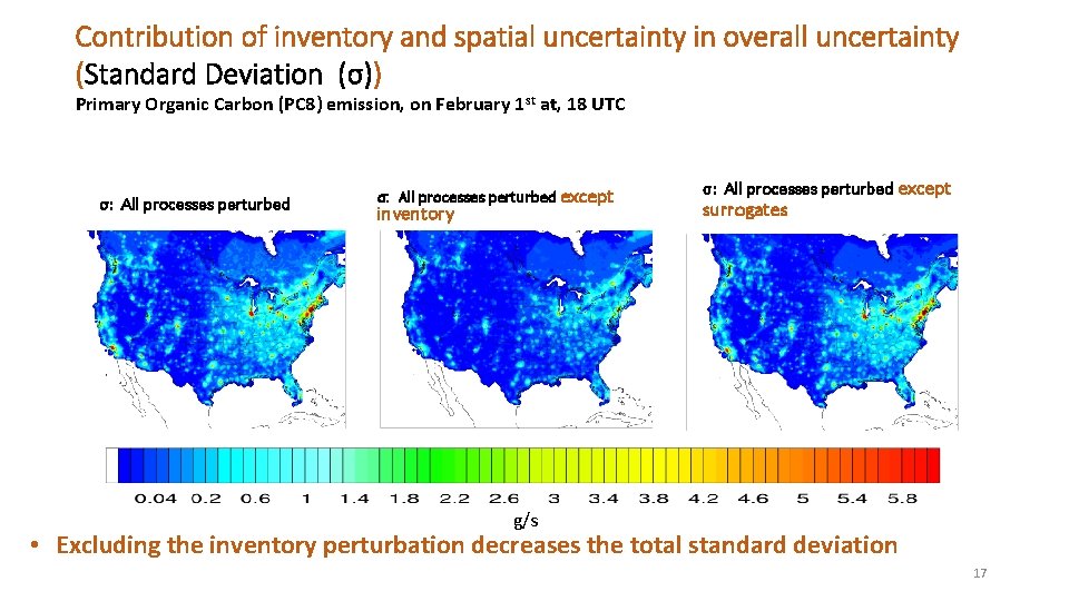
Contribution of inventory and spatial uncertainty in overall uncertainty (Standard Deviation (σ)) Primary Organic Carbon (PC 8) emission, on February 1 st at, 18 UTC σ: All processes perturbed except inventory σ: All processes perturbed except surrogates g/s • Excluding the inventory perturbation decreases the total standard deviation 17

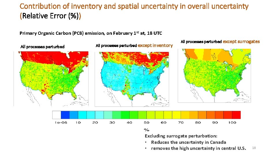
Contribution of inventory and spatial uncertainty in overall uncertainty (Relative Error (%)) Primary Organic Carbon (PC 8) emission, on February 1 st at, 18 UTC All processes perturbed except inventory All processes perturbed except surrogates Excluding surrogate perturbation: • Reduces the uncertainty in Canada • removes the high uncertainty in central U. S. 18

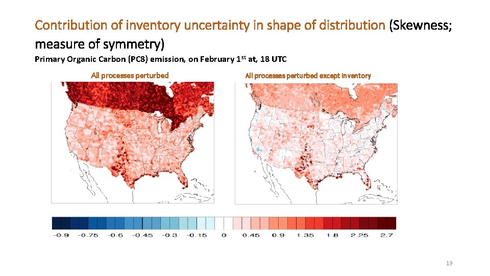
Contribution of inventory uncertainty in shape of distribution (Skewness; measure of symmetry) Primary Organic Carbon (PC 8) emission, on February 1 st at, 18 UTC All processes perturbed except inventory 19

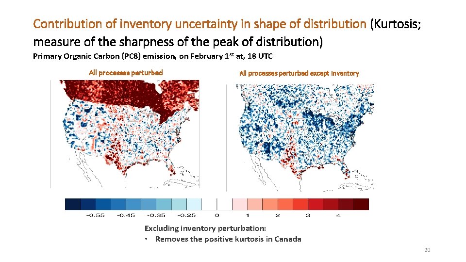
Contribution of inventory uncertainty in shape of distribution (Kurtosis; measure of the sharpness of the peak of distribution) Primary Organic Carbon (PC 8) emission, on February 1 st at, 18 UTC All processes perturbed except inventory Excluding inventory perturbation: • Removes the positive kurtosis in Canada 20

Main Findings: • Emission Inventory is a significant contributor to overall RWC uncertainty • Uncertainty in inventory has also important impact on shape of distribution (both symmetry and sharpness of distribution) • Higher uncertainty in Canada is due to more uncertain input data, especially for inventory parameters, and larger reporting jurisdictions 21

By applying this framework we can: • Generate a set of random realizations of model-ready emission input files, propagate through CTMs • Provide an effective means formal quantification of uncertainties in emissions from other source sectors • Identify gaps in available information for raw emission uncertainty 22

Future steps • Refining RWC emission estimation by including all wood appliance types (e. g. outdoor appliances) • Expanding the framework to other emission sectors (e. g. Road dust) • Propagating emission uncertainties through AQMs (e. g. GEM-MACH) 23

Acknowledgement Thanks to Environment Canada for providing funding for this project 24

THANK YOU 25

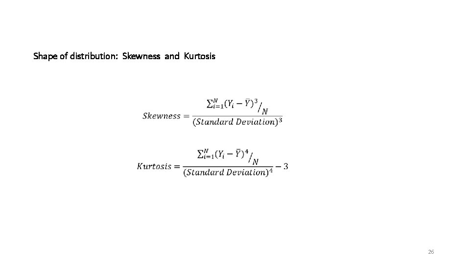
Shape of distribution: Skewness and Kurtosis 26

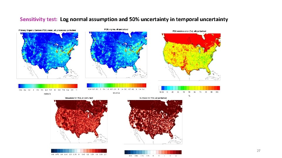
Sensitivity test: Log normal assumption and 50% uncertainty in temporal uncertainty 27

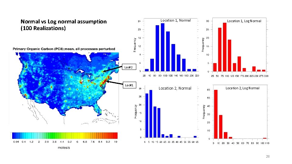
Normal vs Log normal assumption (100 Realizations) Location 1, Normal Location 1, Log Normal Loc#2 Loc#1 Location 2, Normal Location 2, Log Normal 28

29

30

31