EE 441 Data Structures Chapter IX Recursion Trees

EE 441 Data Structures Chapter IX Recursion, Trees Özgür B. Akan Department of Electrical & Electronics Engineering Middle East Technical University akan@eee. metu. edu. tr www. eee. metu. edu. tr/~akan

Recursive Functions n Some calculations have recursive character: n n For example, N!=N*(N-1)! To be able to implement such algorithms, we write functions that call themselves, i. e. , recursive functions n Recursion n n ÖBA’ 2007 Method/Function calls itself Each call is closer to “Base Case” n Base Case == Termination Condition Each call == Loop iteration Each call subject to “stacking” EE-441 Data Structures 2

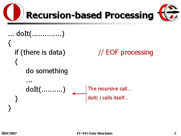
Recursion-based Processing. . . do. It(. . . ) { if (there is data) { do something. . . do. It(. . ) } } ÖBA’ 2007 // EOF processing The recursive call. . . do. It( ) calls itself. . . EE-441 Data Structures 3

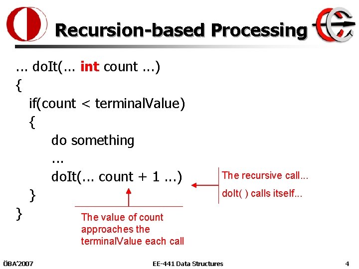
Recursion-based Processing. . . do. It(. . . int count. . . ) { if(count < terminal. Value) { do something. . . do. It(. . . count + 1. . . ) } } The value of count The recursive call. . . do. It( ) calls itself. . . approaches the terminal. Value each call ÖBA’ 2007 EE-441 Data Structures 4

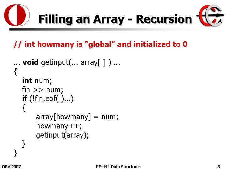
Filling an Array - Recursion // int howmany is “global” and initialized to 0. . . void getinput(. . . array[ ] ). . . { int num; fin >> num; if (!fin. eof( ). . . ) { array[howmany] = num; howmany++; getinput(array); } } ÖBA’ 2007 EE-441 Data Structures 5

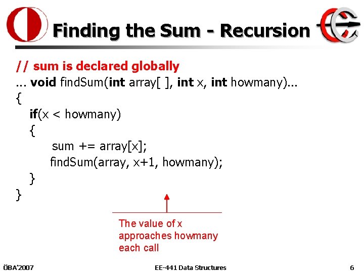
Finding the Sum - Recursion // sum is declared globally. . . void find. Sum(int array[ ], int x, int howmany). . . { if(x < howmany) { sum += array[x]; find. Sum(array, x+1, howmany); } } The value of x approaches howmany each call ÖBA’ 2007 EE-441 Data Structures 6

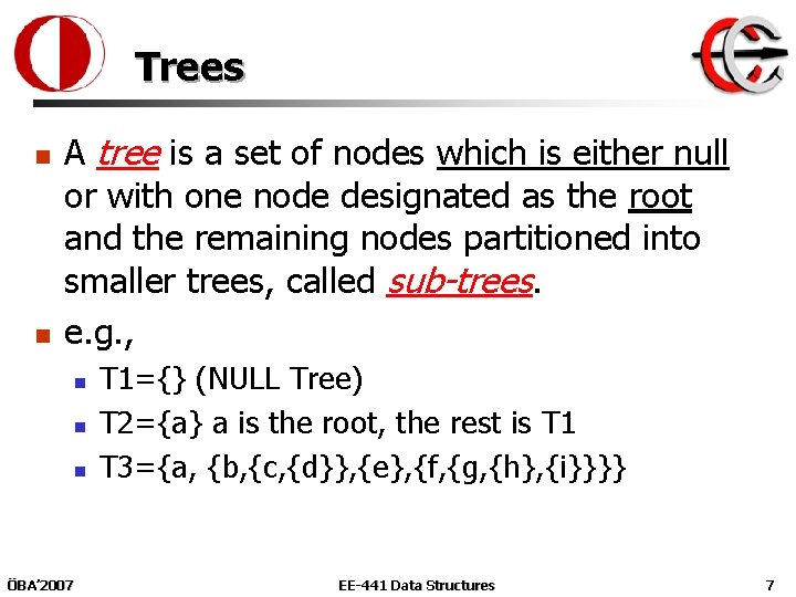
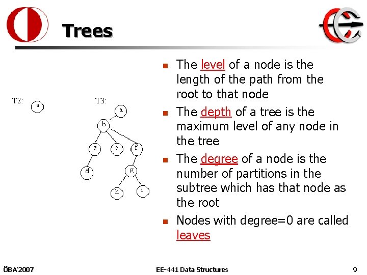
Trees n n A tree is a set of nodes which is either null or with one node designated as the root and the remaining nodes partitioned into smaller trees, called sub-trees. e. g. , n n n ÖBA’ 2007 T 1={} (NULL Tree) T 2={a} a is the root, the rest is T 1 T 3={a, {b, {c, {d}}, {e}, {f, {g, {h}, {i}}}} EE-441 Data Structures 7

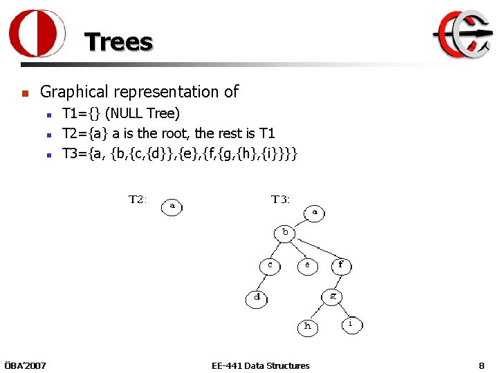
Trees n Graphical representation of n n n ÖBA’ 2007 T 1={} (NULL Tree) T 2={a} a is the root, the rest is T 1 T 3={a, {b, {c, {d}}, {e}, {f, {g, {h}, {i}}}} EE-441 Data Structures 8

Trees n n ÖBA’ 2007 The level of a node is the length of the path from the root to that node The depth of a tree is the maximum level of any node in the tree The degree of a node is the number of partitions in the subtree which has that node as the root Nodes with degree=0 are called leaves EE-441 Data Structures 9

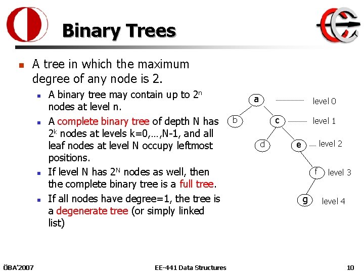
Binary Trees n A tree in which the maximum degree of any node is 2. n n ÖBA’ 2007 A binary tree may contain up to 2 n nodes at level n. A complete binary tree of depth N has 2 k nodes at levels k=0, …, N-1, and all leaf nodes at level N occupy leftmost positions. If level N has 2 N nodes as well, then the complete binary tree is a full tree. If all nodes have degree=1, the tree is a degenerate tree (or simply linked list) EE-441 Data Structures a level 0 c b d level 1 e level 2 f g level 3 level 4 10

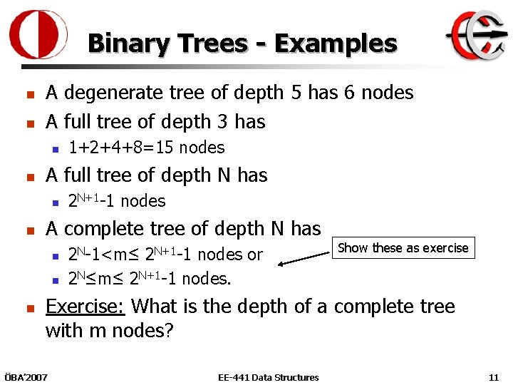
Binary Trees - Examples n n A degenerate tree of depth 5 has 6 nodes A full tree of depth 3 has n n A full tree of depth N has n n 2 N+1 -1 nodes A complete tree of depth N has n n n 1+2+4+8=15 nodes 2 N-1<m≤ 2 N+1 -1 nodes or 2 N≤m≤ 2 N+1 -1 nodes. Show these as exercise Exercise: What is the depth of a complete tree with m nodes? ÖBA’ 2007 EE-441 Data Structures 11

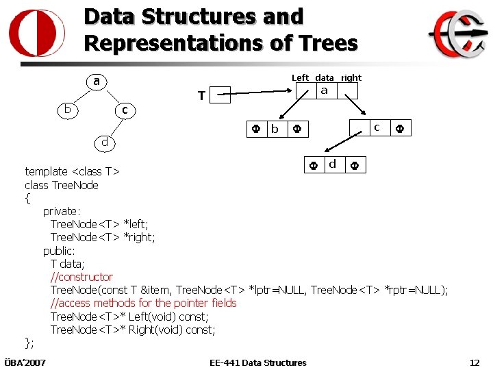
Data Structures and Representations of Trees a Left data right c b a T b c d d template <class T> class Tree. Node { private: Tree. Node<T> *left; Tree. Node<T> *right; public: T data; //constructor Tree. Node(const T &item, Tree. Node<T> *lptr=NULL, Tree. Node<T> *rptr=NULL); //access methods for the pointer fields Tree. Node<T>* Left(void) const; Tree. Node<T>* Right(void) const; }; ÖBA’ 2007 EE-441 Data Structures 12

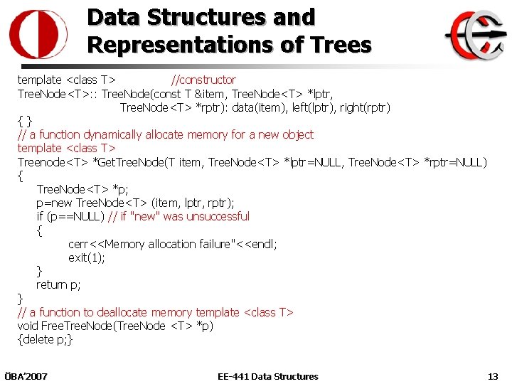
Data Structures and Representations of Trees template <class T> //constructor Tree. Node<T>: : Tree. Node(const T &item, Tree. Node<T> *lptr, Tree. Node<T> *rptr): data(item), left(lptr), right(rptr) {} // a function dynamically allocate memory for a new object template <class T> Treenode<T> *Get. Tree. Node(T item, Tree. Node<T> *lptr=NULL, Tree. Node<T> *rptr=NULL) { Tree. Node<T> *p; p=new Tree. Node<T> (item, lptr, rptr); if (p==NULL) // if "new" was unsuccessful { cerr<<Memory allocation failure"<<endl; exit(1); } return p; } // a function to deallocate memory template <class T> void Free. Tree. Node(Tree. Node <T> *p) {delete p; } ÖBA’ 2007 EE-441 Data Structures 13

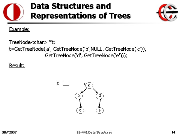
Data Structures and Representations of Trees Example: Tree. Node<char> *t; t=Get. Tree. Node('a', Get. Tree. Node('b', NULL, Get. Tree. Node('c')), Get. Tree. Node('d', Get. Tree. Node('e'))); Result: t ÖBA’ 2007 a b d c e EE-441 Data Structures 14

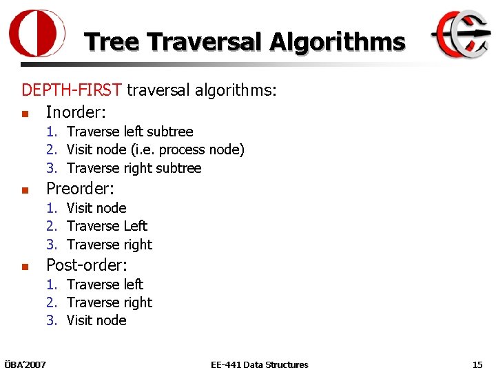
Tree Traversal Algorithms DEPTH-FIRST traversal algorithms: n Inorder: 1. Traverse left subtree 2. Visit node (i. e. process node) 3. Traverse right subtree n Preorder: 1. Visit node 2. Traverse Left 3. Traverse right n Post-order: 1. Traverse left 2. Traverse right 3. Visit node ÖBA’ 2007 EE-441 Data Structures 15

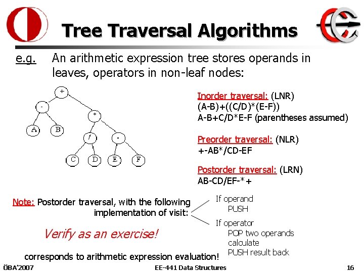
Tree Traversal Algorithms e. g. An arithmetic expression tree stores operands in leaves, operators in non-leaf nodes: Inorder traversal: (LNR) (A-B)+((C/D)*(E-F)) A-B+C/D*E-F (parentheses assumed) Preorder traversal: (NLR) +-AB*/CD-EF Postorder traversal: (LRN) AB-CD/EF-*+ Note: Postorder traversal, with the following implementation of visit: Verify as an exercise! If operand PUSH If operator POP two operands calculate PUSH result back corresponds to arithmetic expression evaluation! ÖBA’ 2007 EE-441 Data Structures 16

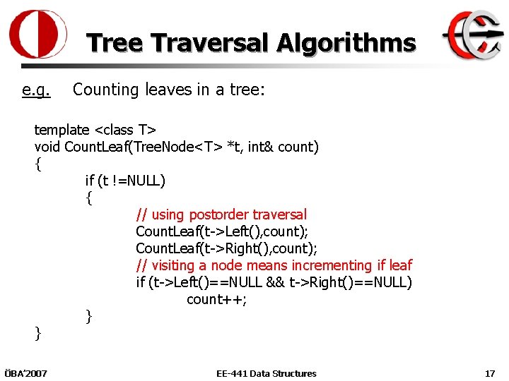
Tree Traversal Algorithms e. g. Counting leaves in a tree: template <class T> void Count. Leaf(Tree. Node<T> *t, int& count) { if (t !=NULL) { // using postorder traversal Count. Leaf(t->Left(), count); Count. Leaf(t->Right(), count); // visiting a node means incrementing if leaf if (t->Left()==NULL && t->Right()==NULL) count++; } } ÖBA’ 2007 EE-441 Data Structures 17

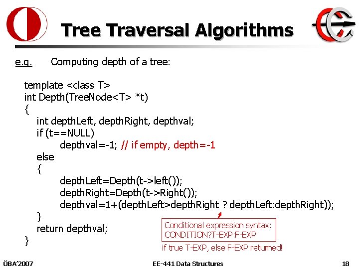
Tree Traversal Algorithms e. g. Computing depth of a tree: template <class T> int Depth(Tree. Node<T> *t) { int depth. Left, depth. Right, depthval; if (t==NULL) depthval=-1; // if empty, depth=-1 else { depth. Left=Depth(t->left()); depth. Right=Depth(t->Right()); depthval=1+(depth. Left>depth. Right ? depth. Left: depth. Right)); } Conditional expression syntax: return depthval; CONDITION? T-EXP: F-EXP } if true T-EXP, else F-EXP returned! ÖBA’ 2007 EE-441 Data Structures 18

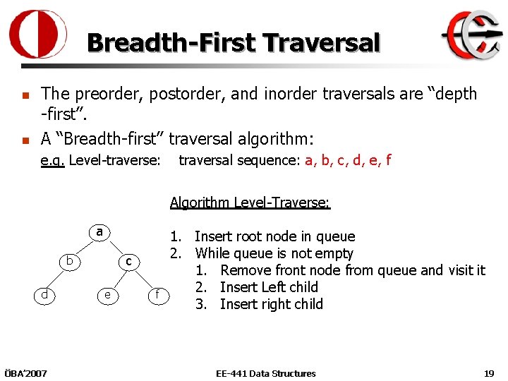
Breadth-First Traversal n n The preorder, postorder, and inorder traversals are “depth -first”. A “Breadth-first” traversal algorithm: e. g. Level-traverse: traversal sequence: a, b, c, d, e, f Algorithm Level-Traverse: a c b d ÖBA’ 2007 e f 1. Insert root node in queue 2. While queue is not empty 1. Remove front node from queue and visit it 2. Insert Left child 3. Insert right child EE-441 Data Structures 19

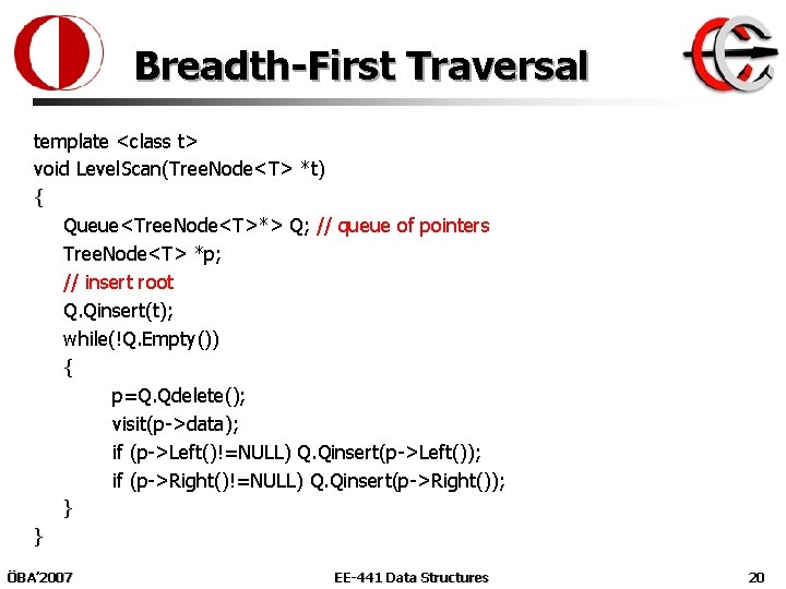
Breadth-First Traversal template <class t> void Level. Scan(Tree. Node<T> *t) { Queue<Tree. Node<T>*> Q; // queue of pointers Tree. Node<T> *p; // insert root Q. Qinsert(t); while(!Q. Empty()) { p=Q. Qdelete(); visit(p->data); if (p->Left()!=NULL) Q. Qinsert(p->Left()); if (p->Right()!=NULL) Q. Qinsert(p->Right()); } } ÖBA’ 2007 EE-441 Data Structures 20

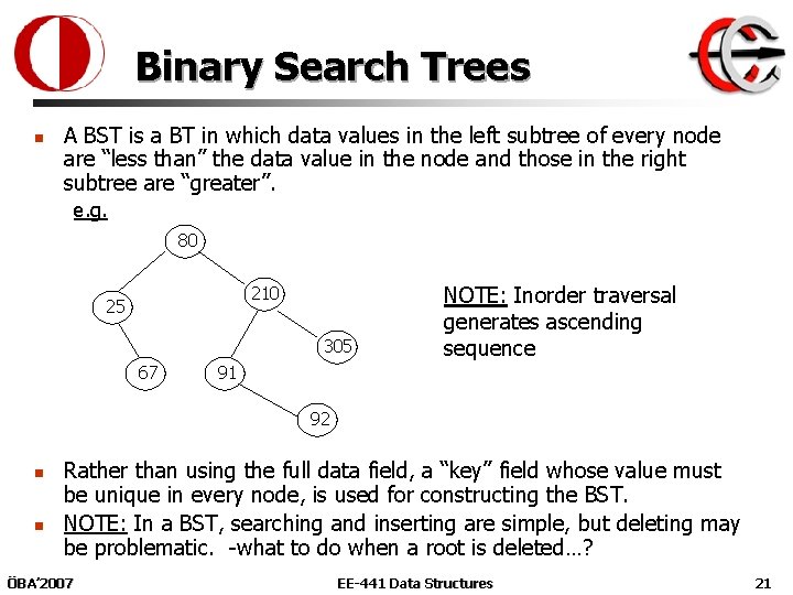
Binary Search Trees n A BST is a BT in which data values in the left subtree of every node are “less than” the data value in the node and those in the right subtree are “greater”. e. g. 80 210 25 305 67 91 NOTE: Inorder traversal generates ascending sequence 92 n n Rather than using the full data field, a “key” field whose value must be unique in every node, is used for constructing the BST. NOTE: In a BST, searching and inserting are simple, but deleting may be problematic. -what to do when a root is deleted…? ÖBA’ 2007 EE-441 Data Structures 21

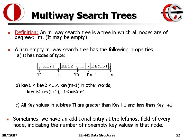
Multiway Search Trees n Definition: An m_way search tree is a tree in which all nodes are of degree<=m. (It may be empty). n A non empty m_way search tree has the following properties: a) It has nodes of type: b) key 1 < key 2 <. . . < key(m-1) in other words, key i< key(i+1), 1<=i<m-1 c) All Key values in subtree Ti are greater than Key i-1 and less than Key i+1 n Sometimes, we have an additional entry at the leftmost field of every node, indicating the number of nonempty key values in that node. ÖBA’ 2007 EE-441 Data Structures 22

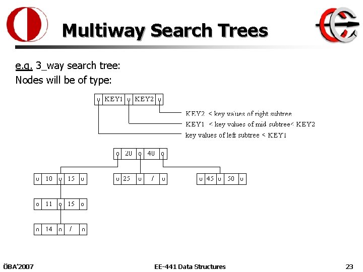
Multiway Search Trees e. g. 3_way search tree: Nodes will be of type: ÖBA’ 2007 EE-441 Data Structures 23

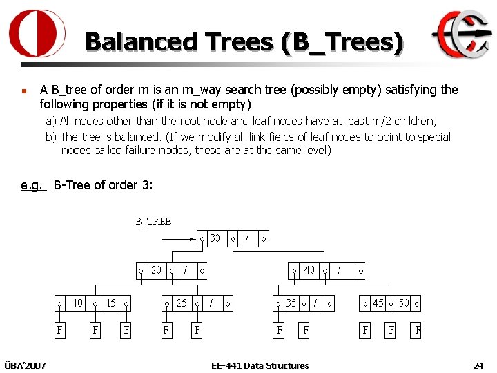
Balanced Trees (B_Trees) n A B_tree of order m is an m_way search tree (possibly empty) satisfying the following properties (if it is not empty) a) All nodes other than the root node and leaf nodes have at least m/2 children, b) The tree is balanced. (If we modify all link fields of leaf nodes to point to special nodes called failure nodes, these are at the same level) e. g. B-Tree of order 3: ÖBA’ 2007 EE-441 Data Structures 24

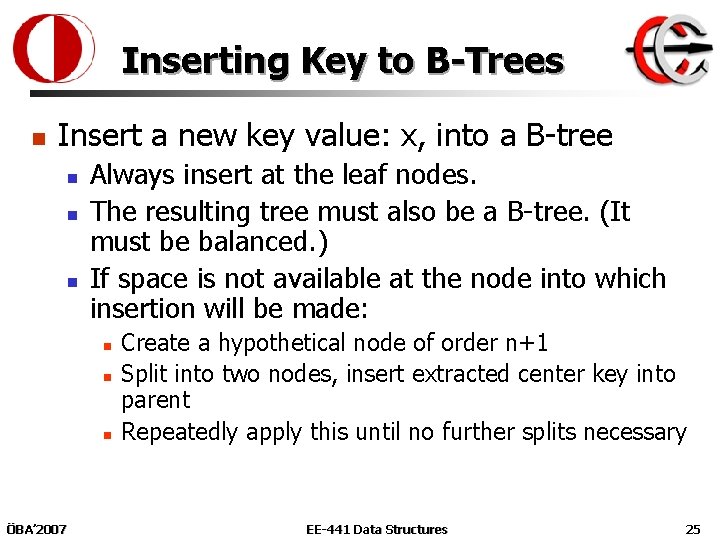
Inserting Key to B-Trees n Insert a new key value: x, into a B-tree n n n Always insert at the leaf nodes. The resulting tree must also be a B-tree. (It must be balanced. ) If space is not available at the node into which insertion will be made: n n n ÖBA’ 2007 Create a hypothetical node of order n+1 Split into two nodes, insert extracted center key into parent Repeatedly apply this until no further splits necessary EE-441 Data Structures 25

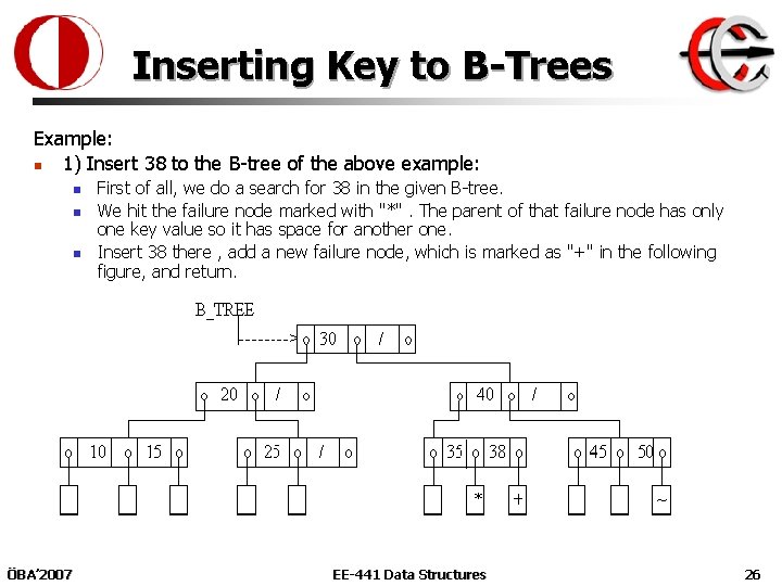
Inserting Key to B-Trees Example: n 1) Insert 38 to the B-tree of the above example: n n n ÖBA’ 2007 First of all, we do a search for 38 in the given B-tree. We hit the failure node marked with "*". The parent of that failure node has only one key value so it has space for another one. Insert 38 there , add a new failure node, which is marked as "+" in the following figure, and return. EE-441 Data Structures 26

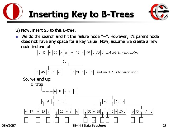
Inserting Key to B-Trees 2) Now, insert 55 to this B-tree. n We do the search and hit the failure node "~". However, it's parent node does not have any space for a key value. Now, assume we create a new node instead of So, we end up: / ÖBA’ 2007 EE-441 Data Structures 27

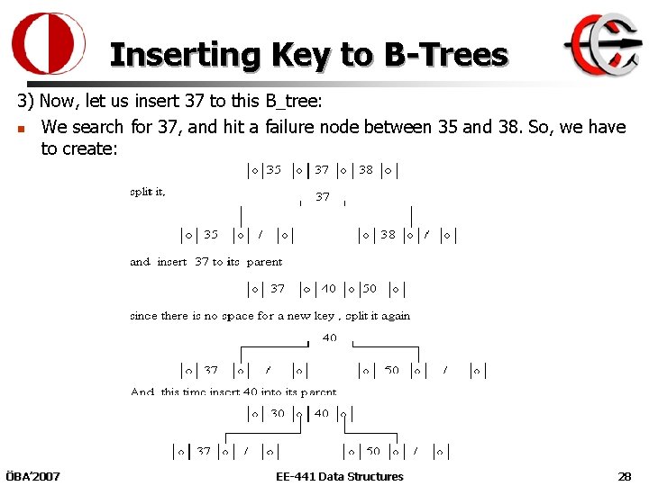
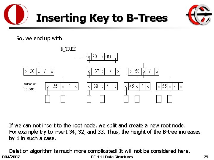
Inserting Key to B-Trees 3) Now, let us insert 37 to this B_tree: n We search for 37, and hit a failure node between 35 and 38. So, we have to create: ÖBA’ 2007 EE-441 Data Structures 28

Inserting Key to B-Trees So, we end up with: 40 If we can not insert to the root node, we split and create a new root node. For example try to insert 34, 32, and 33. Thus, the height of the B-tree increases by 1 in such a case. Deletion algorithm is much more complicated! It will not be considered here. ÖBA’ 2007 EE-441 Data Structures 29