Design and Analysis of Genomewide Association Studies David

Design and Analysis of Genomewide Association Studies David Evans

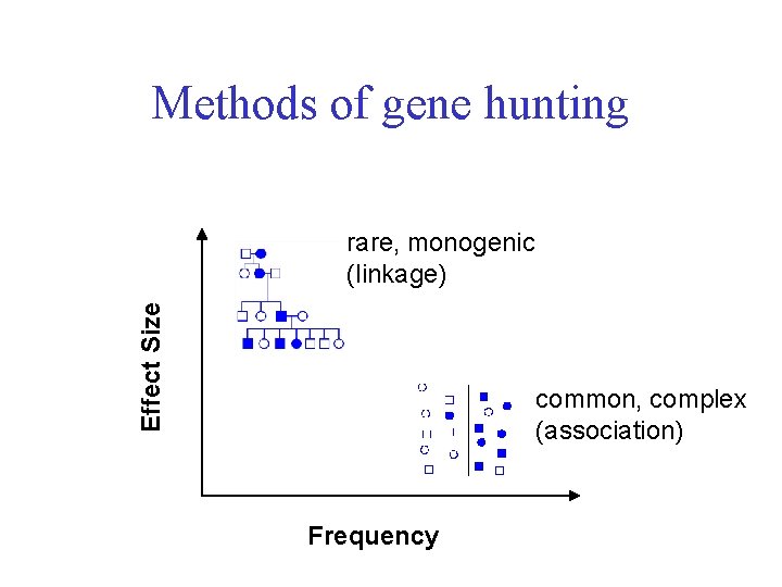
Methods of gene hunting Effect Size rare, monogenic (linkage) common, complex (association) Frequency

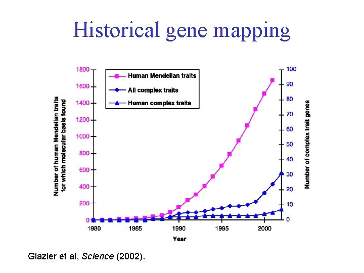
Historical gene mapping Glazier et al, Science (2002).

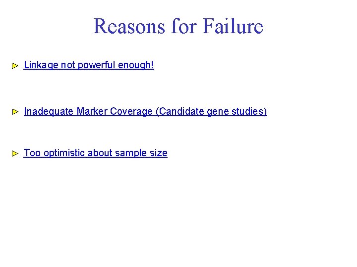
Reasons for Failure Linkage not powerful enough! Inadequate Marker Coverage (Candidate gene studies) Too optimistic about sample size

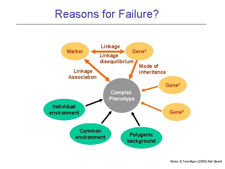
Reasons for Failure? Marker Linkage Gene 1 Linkage disequilibrium Linkage Association Mode of inheritance Gene 2 Complex Phenotype Individual environment Common environment Gene 3 Polygenic background Weiss & Terwilliger (2000) Nat Genet

Enabling Genome-wide Association Studies HAPlotype MAP High throughput genotyping Large cohorts

Wellcome Trust Case Control Consortium

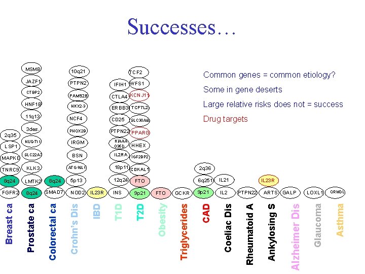
MSMB 10 q 21 JAZF 1 PTPN 2 IFIH 1 WFS 1 FAM 92 B CTLA 4 KCNJ 11 NKX 2 -3 ERBB 3 TCF 7 L 2 Large relative risks does not = success NCF 4 CD 25 Drug targets 3 des. PHOX 2 B PTPN 22 PPARG NUDT 11 IRGM KIAAA 035 D SLC 22 A 3 BSN IL 2 RA IGF 2 BP 2 TNRC 9 KLK 3 ATG 16 L 1 18 p 11 CDKAL 1 2 q 36 8 q 24 LMTK 2 8 q 24 5 p 13 12 q 24 FTO 6 q 251 IL 21 FGFR 2 8 q 24 SMAD 7 NOD 2 IL 23 R INS 9 p 21 FTO GCKR 9 p 21 IL 2 Prostate ca Colorectal ca Crohn’s Dis IBD T 1 D T 2 D Obesity Triglycerides Successes… PTPN 22 ARTS GALP LOXL 1 ORMDL Asthma IL 23 R Glaucoma Breast ca MAPKI 3 HHEX Alzheimer Dis LSP 1 Ankylosing S 2 q 35 SLC 30 A 8 Rheumatoid A 11 q 13 Some in gene deserts Coeliac Dis HNF 1 B Common genes = common etiology? CAD CTBP 2 TCF 2

Study Design

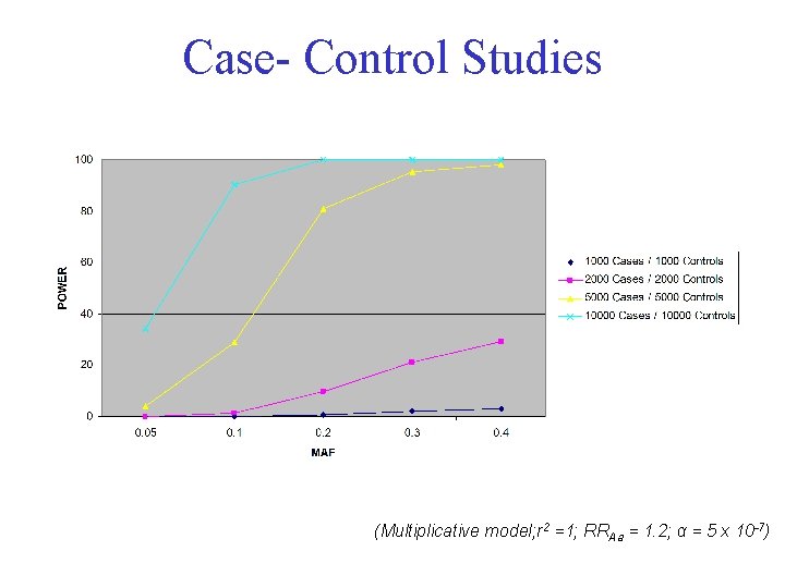
Case- Control Studies (Multiplicative model; r 2 =1; RRAa = 1. 2; α = 5 x 10 -7)

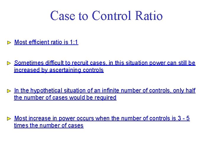
Case to Control Ratio Most efficient ratio is 1: 1 Sometimes difficult to recruit cases, in this situation power can still be increased by ascertaining controls In the hypothetical situation of an infinite number of controls, only half the number of cases would be required Most increase in power occurs when the number of controls is 3 - 5 times the number of cases

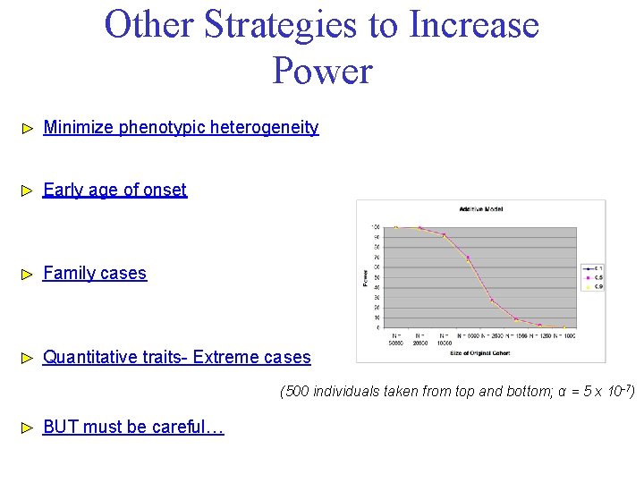
Other Strategies to Increase Power Minimize phenotypic heterogeneity Early age of onset Family cases Quantitative traits- Extreme cases (500 individuals taken from top and bottom; α = 5 x 10 -7) BUT must be careful…

Phenotypic Misclassification in psychiatric genetics Random misclassification should not affect type I error but will decrease power Misclassifying cases is not the same as misclassifying controls. The effect of each depends on the prevalence of disease For example, for diseases where prevalence less than 10% much more important to ensure cases are truly affected than controls are really unaffected Use of historic controls (but note stratification; batch effects; platform differences)

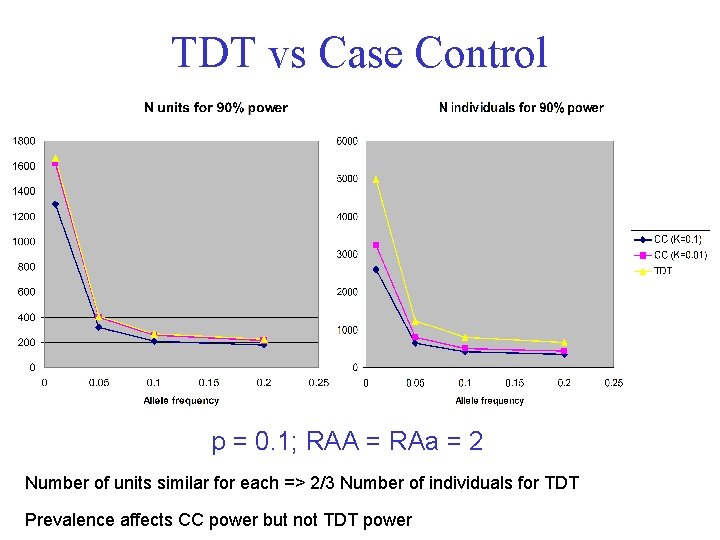
TDT vs Case Control p = 0. 1; RAA = RAa = 2 Number of units similar for each => 2/3 Number of individuals for TDT Prevalence affects CC power but not TDT power

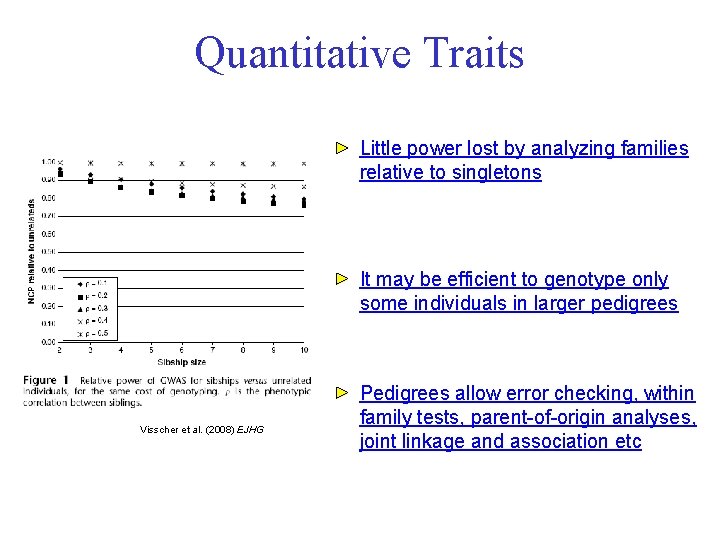
Quantitative Traits Little power lost by analyzing families relative to singletons It may be efficient to genotype only some individuals in larger pedigrees Visscher et al. (2008) EJHG Pedigrees allow error checking, within family tests, parent-of-origin analyses, joint linkage and association etc

Genotyping Platform

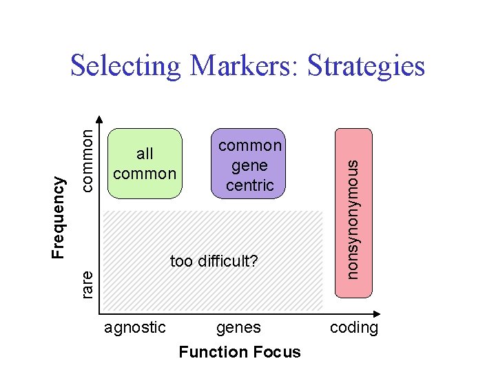
common gene centric too difficult? agnostic genes Function Focus nonsynonymous common all common rare Frequency Selecting Markers: Strategies coding

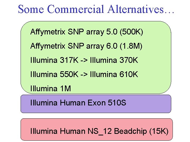
Some Commercial Alternatives… Affymetrix SNP array 5. 0 (500 K) Affymetrix SNP array 6. 0 (1. 8 M) Illumina 317 K -> Illumina 370 K Illumina 550 K -> Illumina 610 K Illumina 1 M Illumina Human Exon 510 S Illumina Human NS_12 Beadchip (15 K)

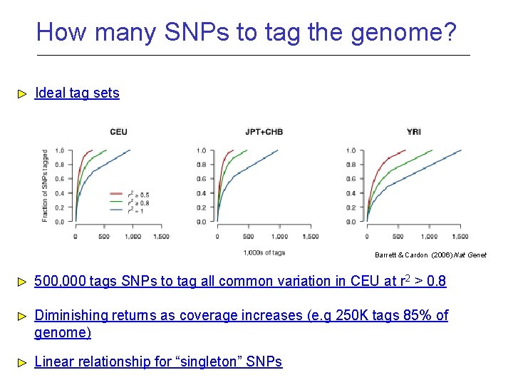
How many SNPs to tag the genome? Ideal tag sets Barrett & Cardon (2006) Nat Genet 500, 000 tags SNPs to tag all common variation in CEU at r 2 > 0. 8 Diminishing returns as coverage increases (e. g 250 K tags 85% of genome) Linear relationship for “singleton” SNPs

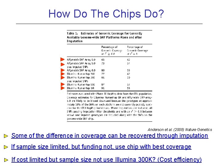
How Do The Chips Do? Anderson et al. (2008) Nature Genetics Some of the difference in coverage can be recovered through imputation If sample size limited, but funding not, use chip with best coverage If cost limited but sample size not use Illumina 300 K? (Cost efficiency)

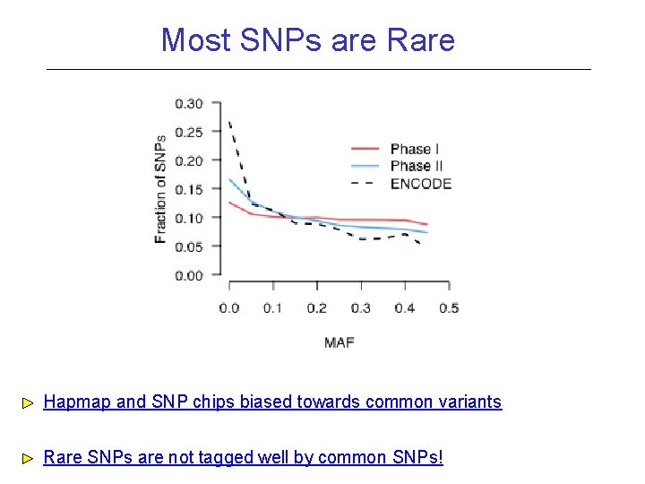
Most SNPs are Rare Hapmap and SNP chips biased towards common variants Rare SNPs are not tagged well by common SNPs!

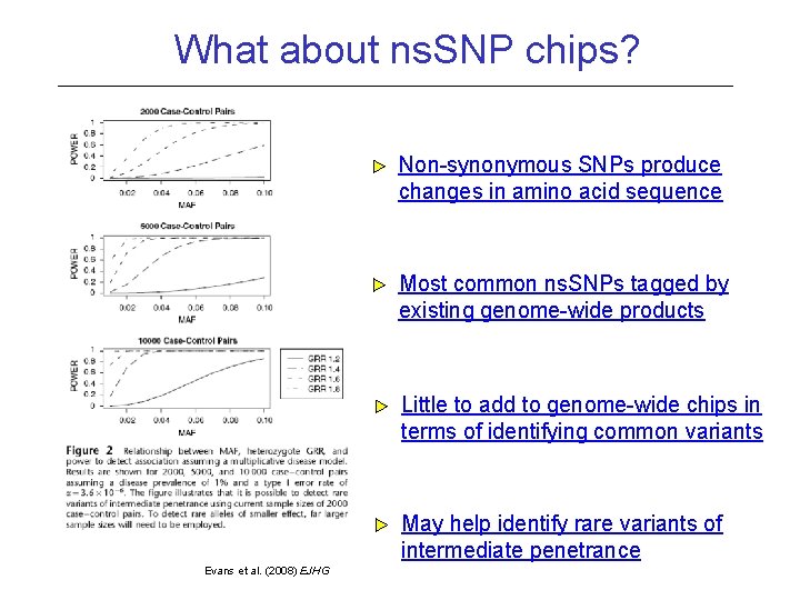
What about ns. SNP chips? Non-synonymous SNPs produce changes in amino acid sequence Most common ns. SNPs tagged by existing genome-wide products Little to add to genome-wide chips in terms of identifying common variants May help identify rare variants of intermediate penetrance Evans et al. (2008) EJHG

“Cleaning” Data

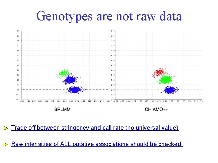
Genotypes are not raw data Trade off between stringency and call rate (no universal value) Raw intensities of ALL putative associations should be checked!

SNP Quality Control Missing Data Rate (SNPs, Individuals, cases vs controls) Hardy Weinberg Equilibrium Allele frequency Mendelian Inconsistencies

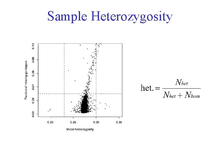
Sample Heterozygosity

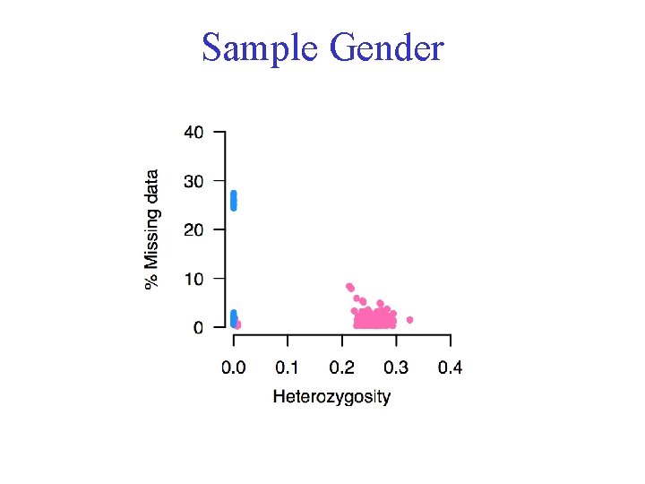
Sample Gender

Association Analysis

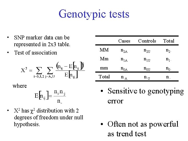
Genotypic tests • SNP marker data can be represented in 2 x 3 table. • Test of association where • X 2 has χ2 distribution with 2 degrees of freedom under null hypothesis. Cases Controls Total MM n 2 A n 2 U n 2· Mm n 1 A n 1 U n 1· mm n 0 A n 0 U n 0· Total n·A n·U n·· • Sensitive to genotyping error • Often not as powerful as trend test

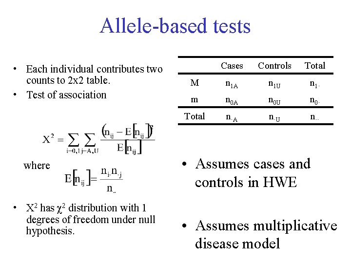
Allele-based tests • Each individual contributes two counts to 2 x 2 table. • Test of association where • X 2 has χ2 distribution with 1 degrees of freedom under null hypothesis. Cases Controls Total M n 1 A n 1 U n 1· m n 0 A n 0 U n 0· Total n·A n·U n·· • Assumes cases and controls in HWE • Assumes multiplicative disease model

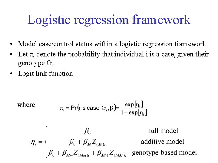
Logistic regression framework • Model case/control status within a logistic regression framework. • Let πi denote the probability that individual i is a case, given their genotype Gi. • Logit link function where

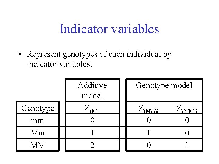
Indicator variables • Represent genotypes of each individual by indicator variables: Genotype mm Mm MM Additive model Z(M)i 0 1 2 Genotype model Z(Mm)i 0 1 0 Z(MM)i 0 0 1

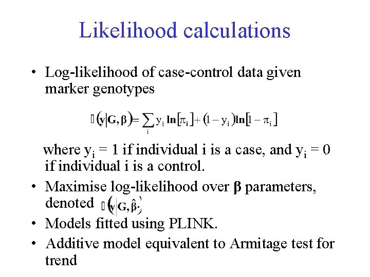
Likelihood calculations • Log-likelihood of case-control data given marker genotypes where yi = 1 if individual i is a case, and yi = 0 if individual i is a control. • Maximise log-likelihood over β parameters, denoted. • Models fitted using PLINK. • Additive model equivalent to Armitage test for trend

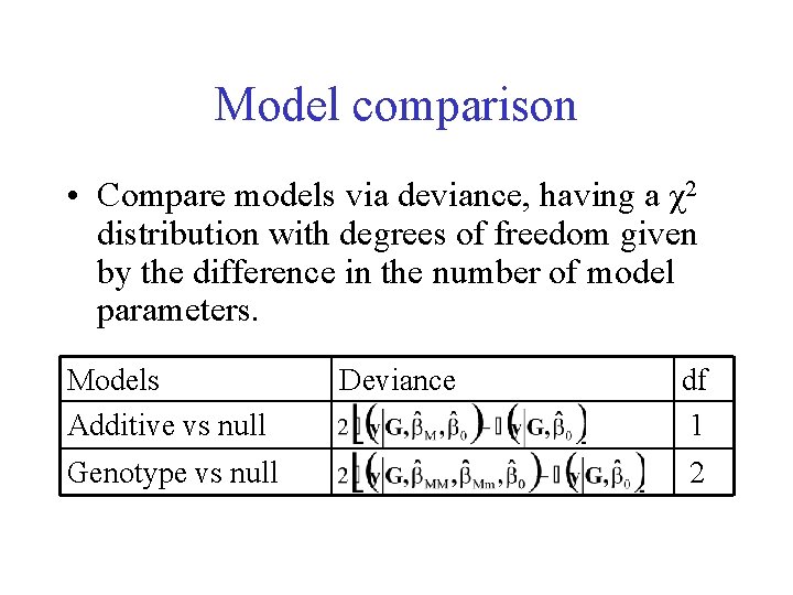
Model comparison • Compare models via deviance, having a χ2 distribution with degrees of freedom given by the difference in the number of model parameters. Models Additive vs null Genotype vs null Deviance df 1 2

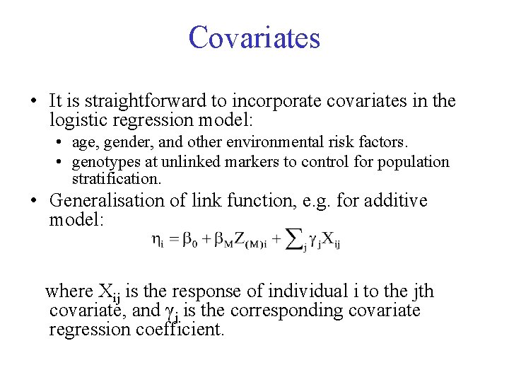
Covariates • It is straightforward to incorporate covariates in the logistic regression model: • age, gender, and other environmental risk factors. • genotypes at unlinked markers to control for population stratification. • Generalisation of link function, e. g. for additive model: where Xij is the response of individual i to the jth covariate, and γj is the corresponding covariate regression coefficient.

Controlling for Population Stratification

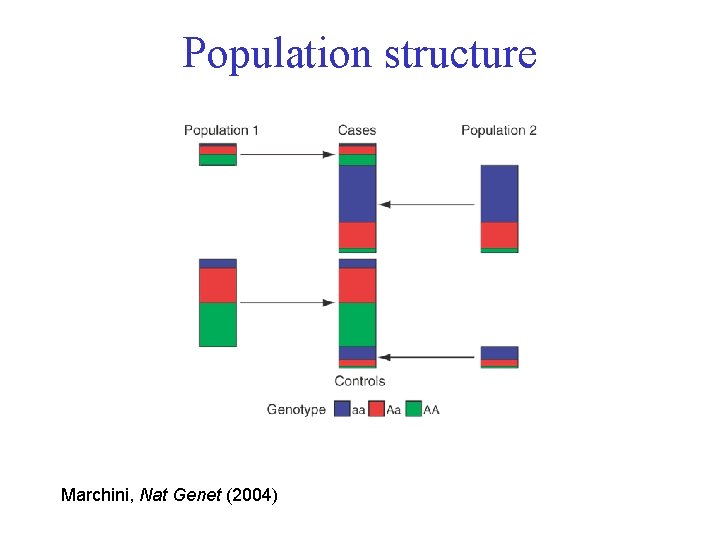
Population structure Marchini, Nat Genet (2004)

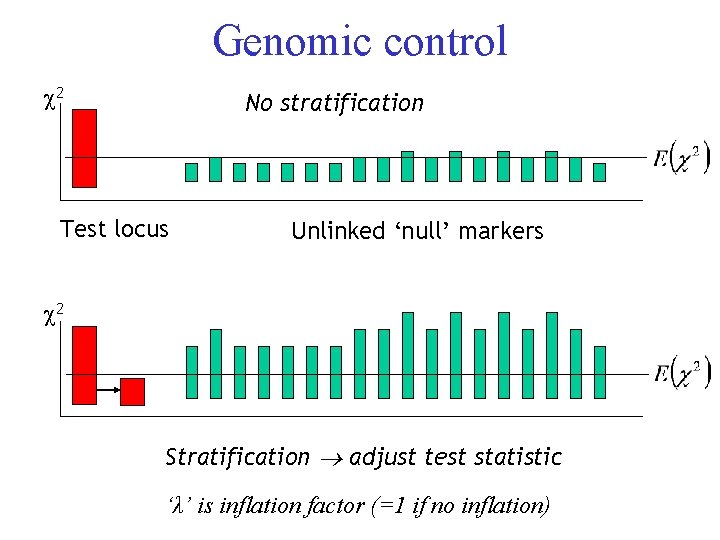
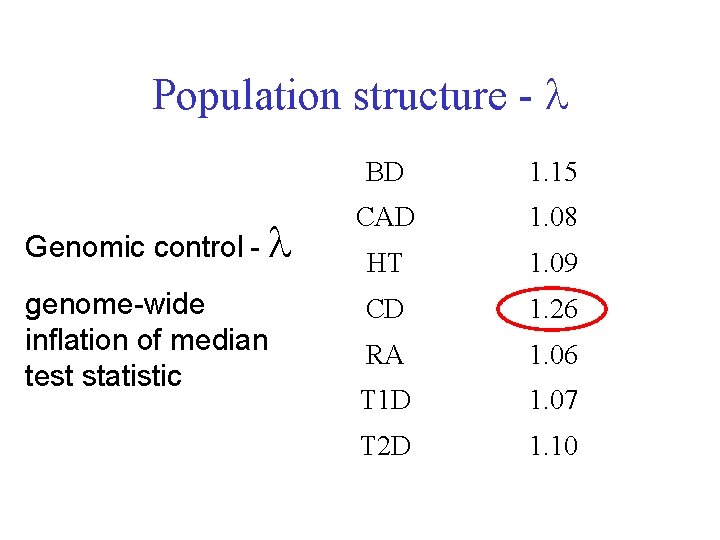
Genomic control 2 No stratification Test locus Unlinked ‘null’ markers 2 Stratification adjust test statistic ‘λ’ is inflation factor (=1 if no inflation)

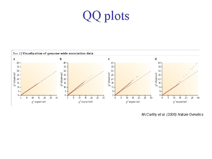
QQ plots Mc. Carthy et al. (2008) Nature Genetics

Population structure - Genomic control - genome-wide inflation of median test statistic BD 1. 15 CAD 1. 08 HT 1. 09 CD 1. 26 RA 1. 06 T 1 D 1. 07 T 2 D 1. 10

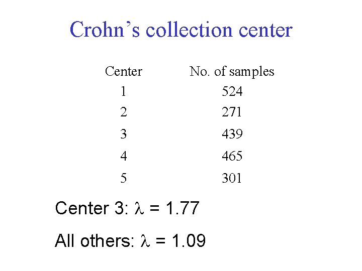
Crohn’s collection center Center 1 2 No. of samples 524 271 3 439 4 465 5 301 Center 3: = 1. 77 All others: = 1. 09

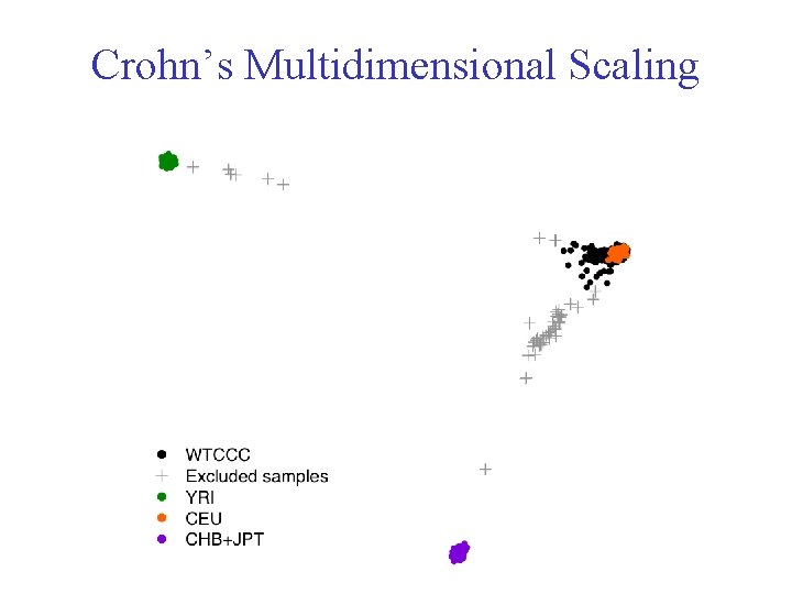
Crohn’s Multidimensional Scaling

Principal Components Analysis • Principal Components Analysis is a data reduction technique where many variables are reduced to a few “principal components”: – Each component describes as much variability as possible – Components are orthogonal and describe consecutively smaller proportions of the variance – First few components reflect population ancestry • Genotypes and phenotypes are adjusted by amounts attributable to ancestry along each component by computing residuals of linear regressions • Association statistics are computed using ancestry adjusted genotypes and phenotypes

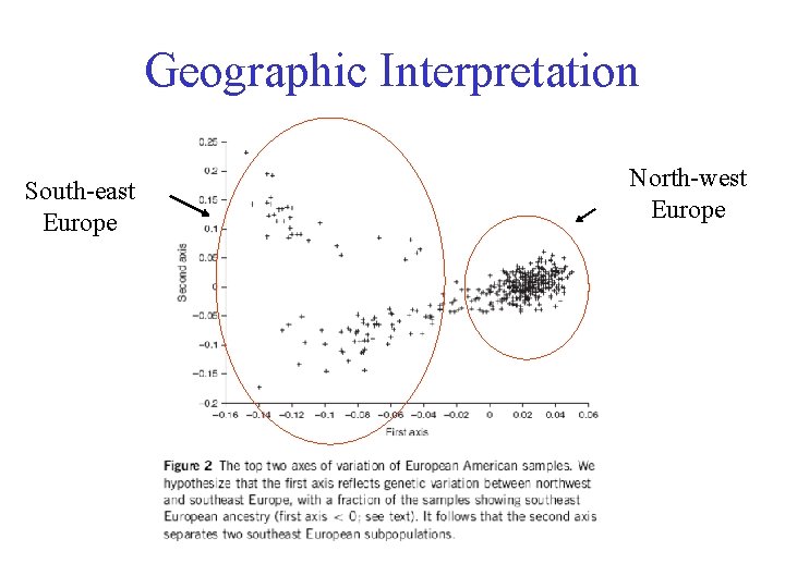
Geographic Interpretation South-east Europe North-west Europe

Imputation

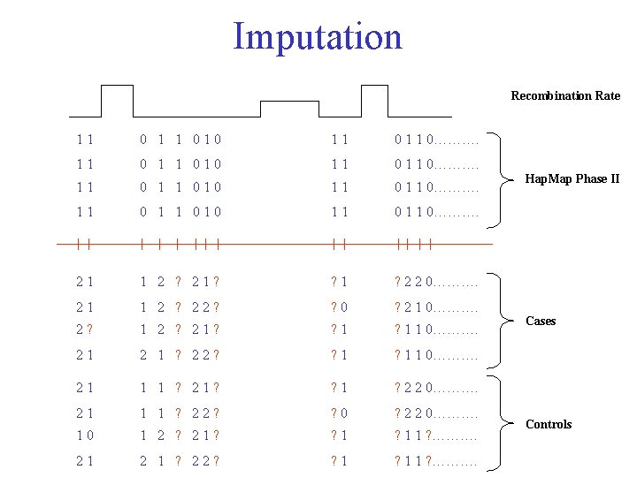
Imputation Recombination Rate 11 0 1 1 010 11 0 1 1 0………. 21 1 2 ? 21? ? 1 ? 2 2 0………. 21 1 2 ? 22? ? 0 ? 2 1 0………. 2? 1 2 ? 21? ? 1 1 0………. 21 2 1 ? 22? ? 1 1 0………. 21 1 1 ? 21? ? 1 ? 2 2 0………. 21 1 1 ? 22? ? 0 ? 2 2 0………. 10 1 2 ? 21? ? 1 1 ? ………. 21 2 1 ? 22? ? 1 1 ? ………. Hap. Map Phase II Cases Controls

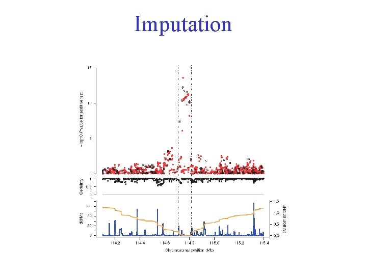
Imputation

Interpretation and Prioritizing SNPs

Asymptotic P values • “The probability of observing the test result or a more extreme value than the test result under the null hypothesis” • The p value is NOT the probability that the null hypothesis is true • The probability that the null/alternate hypothesis is true is a function of the evidence contained in the data (p value), the power of the test, and the prior probability that the association is true/false • The p value is a fluid measure of the strength of evidence against the null hypothesis that was designed to be interpreted in conjunction with other (pre-existing) evidence

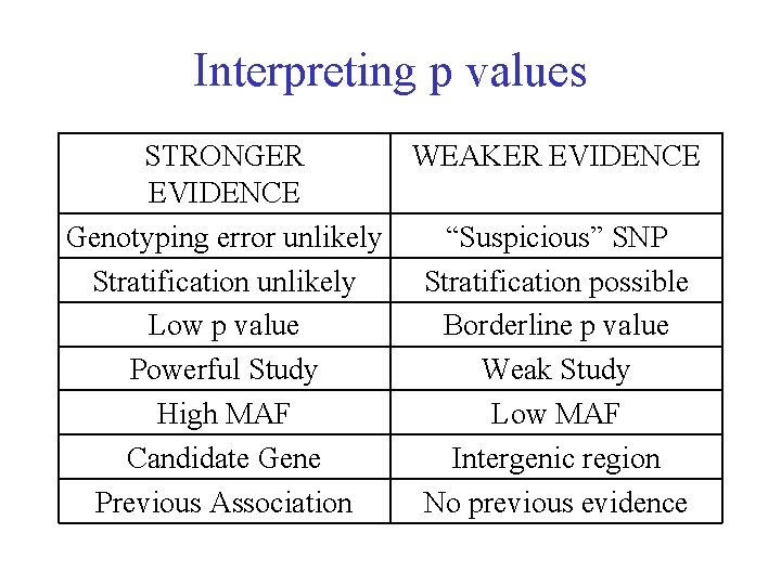
Interpreting p values STRONGER WEAKER EVIDENCE Genotyping error unlikely “Suspicious” SNP Stratification unlikely Stratification possible Low p value Borderline p value Powerful Study Weak Study High MAF Low MAF Candidate Gene Intergenic region Previous Association No previous evidence

Criticisms of p values • Doesn’t formally incorporate prior information • Discards information on the power of the test • Does not take into account the size of the observed effect • Ranking SNPs by p value is problematic!!!

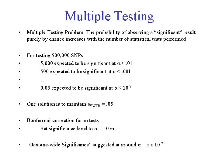
Multiple Testing • Multiple Testing Problem: The probability of observing a “significant” result purely by chance increases with the number of statistical tests performed • • • For testing 500, 000 SNPs 5, 000 expected to be significant at α <. 01 500 expected to be significant at α <. 001 … 0. 05 expected to be significant at α < 10 -7 • One solution is to maintain αFWER =. 05 • • Bonferroni correction for m tests Set significance level to α =. 05/m • “Genome-wide Significance” suggested at around α = 5 x 10 -7

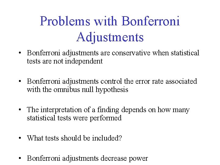
Problems with Bonferroni Adjustments • Bonferroni adjustments are conservative when statistical tests are not independent • Bonferroni adjustments control the error rate associated with the omnibus null hypothesis • The interpretation of a finding depends on how many statistical tests were performed • What tests should be included? • Bonferroni adjustments decrease power

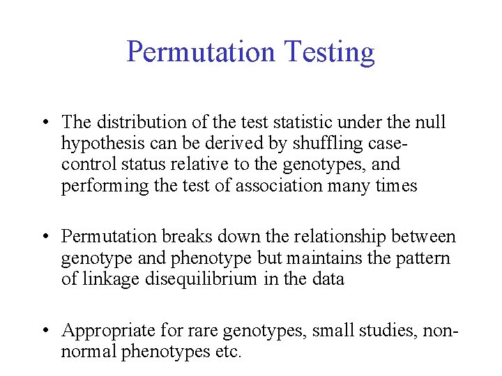
Permutation Testing • The distribution of the test statistic under the null hypothesis can be derived by shuffling casecontrol status relative to the genotypes, and performing the test of association many times • Permutation breaks down the relationship between genotype and phenotype but maintains the pattern of linkage disequilibrium in the data • Appropriate for rare genotypes, small studies, nonnormal phenotypes etc.

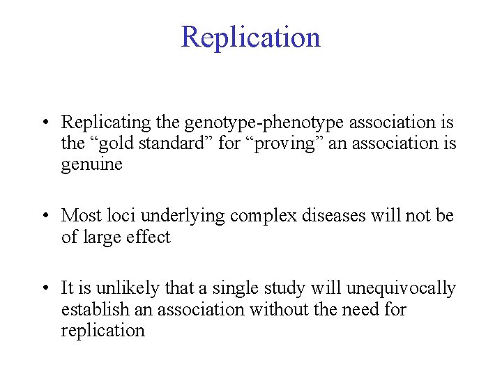
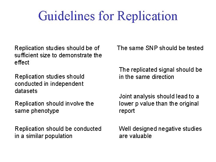
Replication • Replicating the genotype-phenotype association is the “gold standard” for “proving” an association is genuine • Most loci underlying complex diseases will not be of large effect • It is unlikely that a single study will unequivocally establish an association without the need for replication

Guidelines for Replication studies should be of sufficient size to demonstrate the effect Replication studies should conducted in independent datasets The same SNP should be tested The replicated signal should be in the same direction Replication should involve the same phenotype Joint analysis should lead to a lower p value than the original report Replication should be conducted in a similar population Well designed negative studies are valuable

Meta-analysis

Meta-analysis

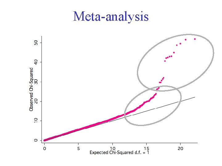
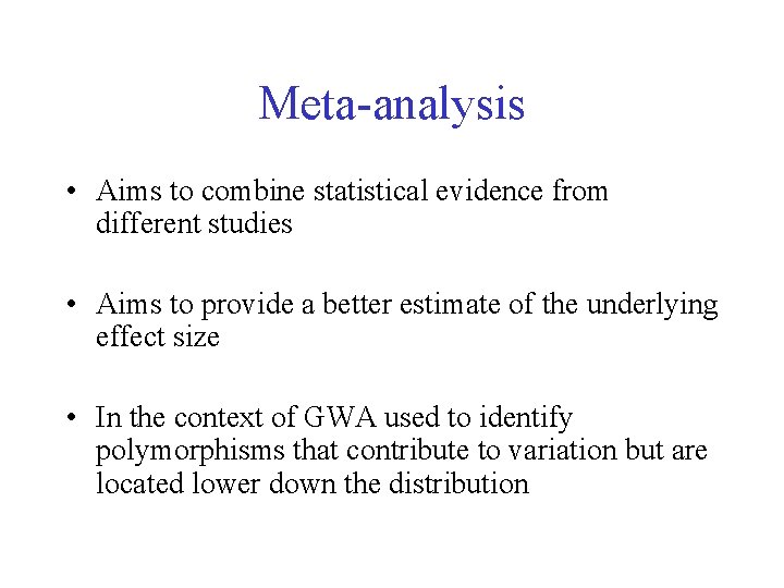
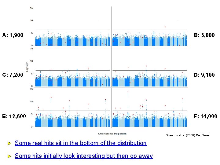
Meta-analysis • Aims to combine statistical evidence from different studies • Aims to provide a better estimate of the underlying effect size • In the context of GWA used to identify polymorphisms that contribute to variation but are located lower down the distribution

Meta-analysis • Larger studies carry more weight • Fixed versus Random Effects • Assessment of Heterogeneity

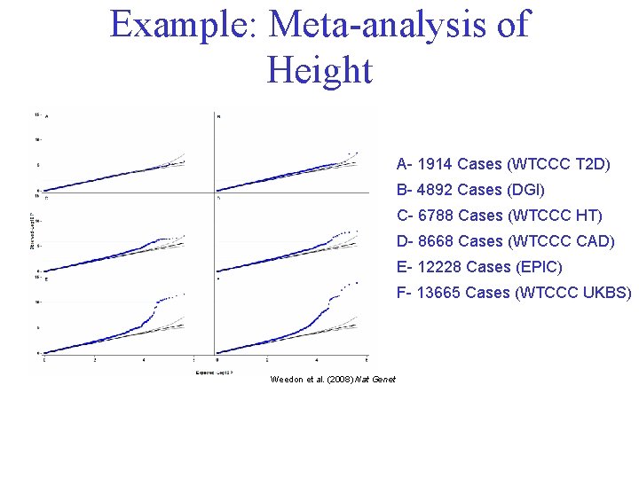
Example: Meta-analysis of Height A- 1914 Cases (WTCCC T 2 D) B- 4892 Cases (DGI) C- 6788 Cases (WTCCC HT) D- 8668 Cases (WTCCC CAD) E- 12228 Cases (EPIC) F- 13665 Cases (WTCCC UKBS) Weedon et al. (2008) Nat Genet

A: 1, 900 B: 5, 000 C: 7, 200 D: 9, 100 E: 12, 600 F: 14, 000 Weedon et al. (2008) Nat Genet Some real hits sit in the bottom of the distribution Some hits initially look interesting but then go away

Statistical Methods for the Analysis of Genome-wide Association Studies Go to: http: //www. hstalks. com