DataFlow Analysis Proving Little Theorems DataFlow Equations Major

Data-Flow Analysis Proving Little Theorems Data-Flow Equations Major Examples 1

An Obvious Theorem boolean x = true; while (x) {. . . // no change to x } u. Doesn’t terminate. u. Proof: only assignment to x is at top, so x is always true. 2

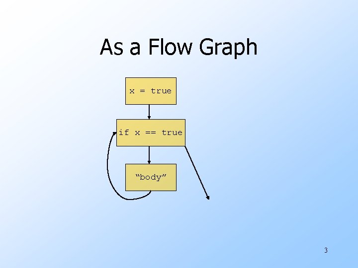
As a Flow Graph x = true if x == true “body” 3

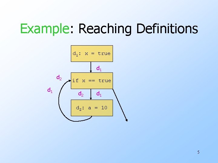
Formulation: Reaching Definitions u. Each place some variable x is assigned is a definition. u. Ask: for this use of x, where could x last have been defined. u. In our example: only at x=true. 4

Example: Reaching Definitions d 1: x = true d 1 d 2 d 1 if x == true d 2 d 1 d 2: a = 10 5

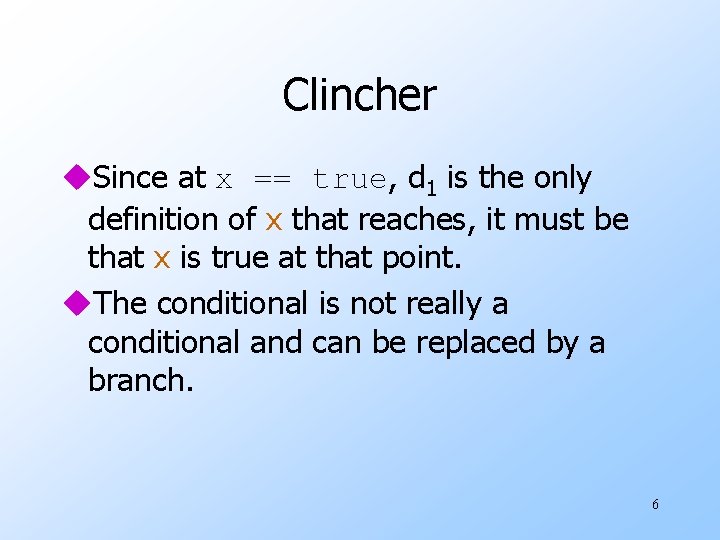
Clincher u. Since at x == true, d 1 is the only definition of x that reaches, it must be that x is true at that point. u. The conditional is not really a conditional and can be replaced by a branch. 6

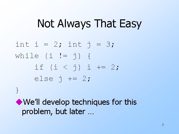
Not Always That Easy int i = 2; int j = 3; while (i != j) { if (i < j) i += 2; else j += 2; } u. We’ll develop techniques for this problem, but later … 7

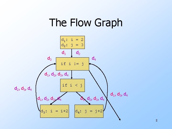
The Flow Graph d 1: i = 2 d 2: j = 3 d 1 d 3 d 2 d 4 if i != j d 1 , d 2 , d 3 , d 4 if i < j d 2 , d 3 , d 4 d 1 , d 2 , d 3 , d 4 d 3: i = i+2 d 1 , d 2 , d 3 , d 4 d 1 , d 3 , d 4: j = j+2 8

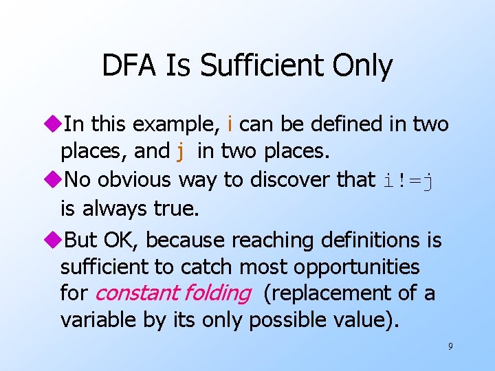
DFA Is Sufficient Only u. In this example, i can be defined in two places, and j in two places. u. No obvious way to discover that i!=j is always true. u. But OK, because reaching definitions is sufficient to catch most opportunities for constant folding (replacement of a variable by its only possible value). 9

Be Conservative! u(Code optimization only) u. It’s OK to discover a subset of the opportunities to make some codeimproving transformation. u. It’s not OK to think you have an opportunity that you don’t really have. 10

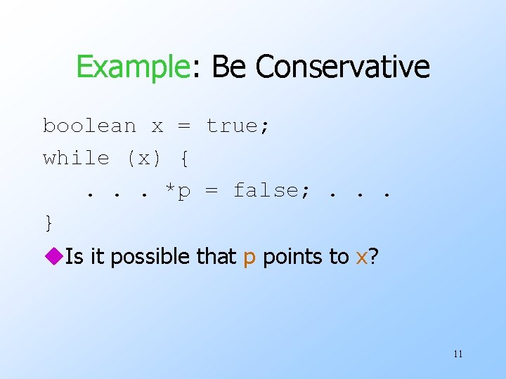
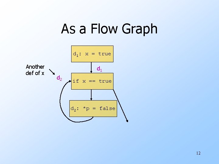
Example: Be Conservative boolean x = true; while (x) {. . . *p = false; . . . } u. Is it possible that p points to x? 11

As a Flow Graph d 1: x = true Another def of x d 1 d 2 if x == true d 2: *p = false 12

Possible Resolution u. Just as data-flow analysis of “reaching definitions” can tell what definitions of x might reach a point, another DFA can eliminate cases where p definitely does not point to x. u. Example: the only definition of p is p = &y and there is no possibility that y is an alias of x. 13

Reaching Definitions Formalized u A definition d of a variable x is said to reach a point p in a flow graph if: 1. Every path from the entry of the flow graph to p has d on the path, and 2. After the last occurrence of d there is no possibility that x is redefined. 14

Data-Flow Equations --- (1) u A basic block can generate a definition. u A basic block can either 1. Kill a definition of x if it surely redefines x. 2. Transmit a definition if it may not redefine the same variable(s) as that definition. 15

Data-Flow Equations --- (2) u Variables: 1. IN(B) = set of definitions reaching the beginning of block B. 2. OUT(B) = set of definitions reaching the end of B. 16

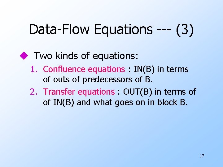
Data-Flow Equations --- (3) u Two kinds of equations: 1. Confluence equations : IN(B) in terms of outs of predecessors of B. 2. Transfer equations : OUT(B) in terms of of IN(B) and what goes on in block B. 17

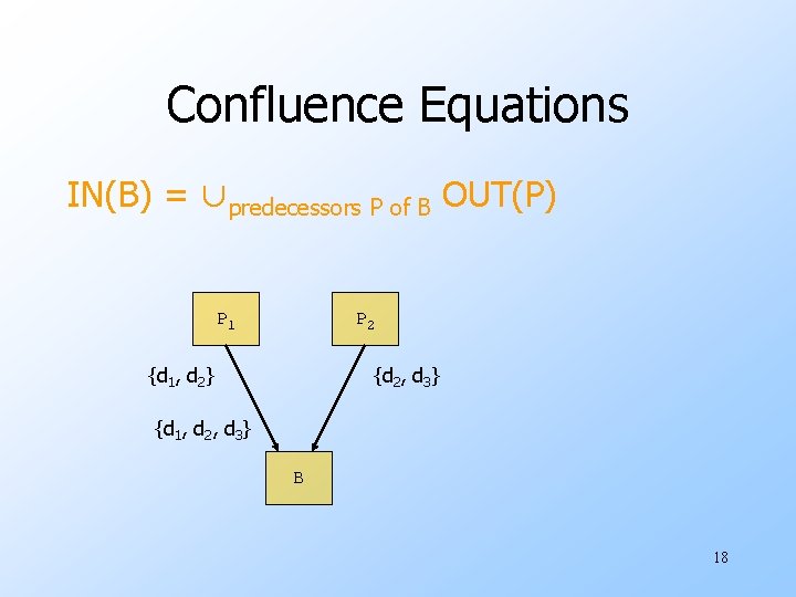
Confluence Equations IN(B) = ∪predecessors P of B OUT(P) P 1 P 2 {d 1, d 2} {d 2, d 3} {d 1, d 2, d 3} B 18

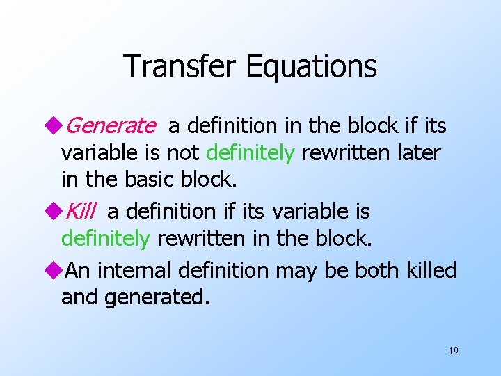
Transfer Equations u. Generate a definition in the block if its variable is not definitely rewritten later in the basic block. u. Kill a definition if its variable is definitely rewritten in the block. u. An internal definition may be both killed and generated. 19

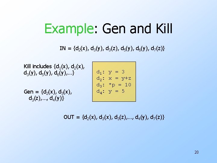
Example: Gen and Kill IN = {d 2(x), d 3(y), d 3(z), d 5(y), d 6(y), d 7(z)} Kill includes {d 1(x), d 2(x), d 3(y), d 5(y), d 6(y), …} Gen = {d 2(x), d 3(z), …, d 4(y)} d 1: d 2: d 3: d 4: y = 3 x = y+z *p = 10 y = 5 OUT = {d 2(x), d 3(z), …, d 4(y), d 7(z)} 20

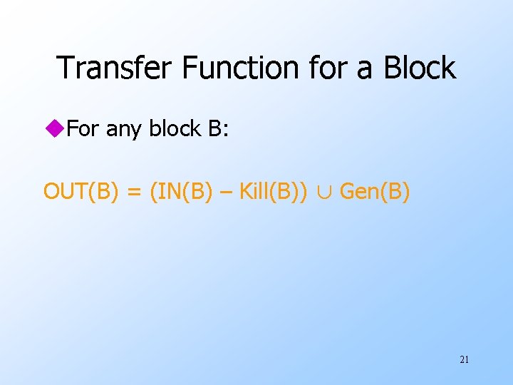
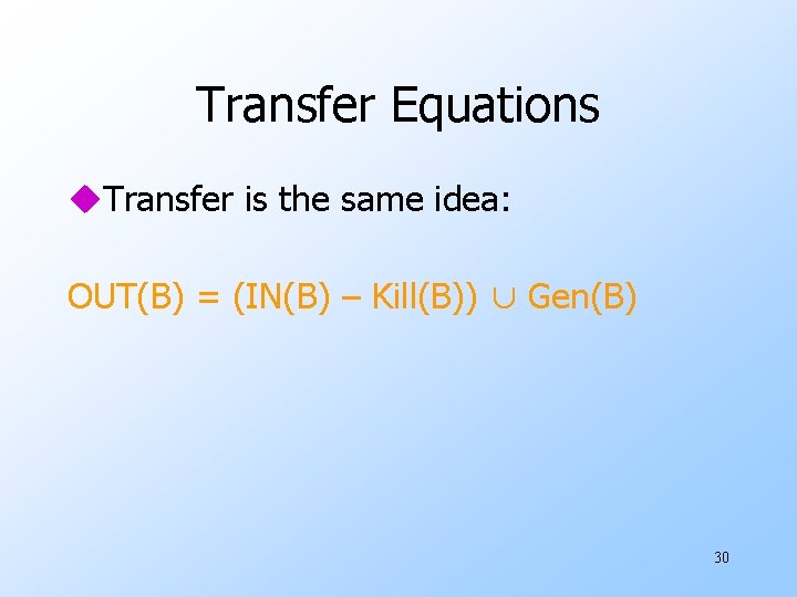
Transfer Function for a Block u. For any block B: OUT(B) = (IN(B) – Kill(B)) ∪ Gen(B) 21

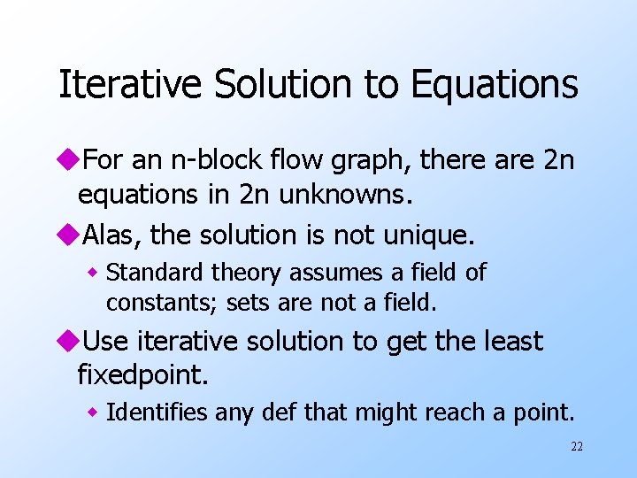
Iterative Solution to Equations u. For an n-block flow graph, there are 2 n equations in 2 n unknowns. u. Alas, the solution is not unique. w Standard theory assumes a field of constants; sets are not a field. u. Use iterative solution to get the least fixedpoint. w Identifies any def that might reach a point. 22

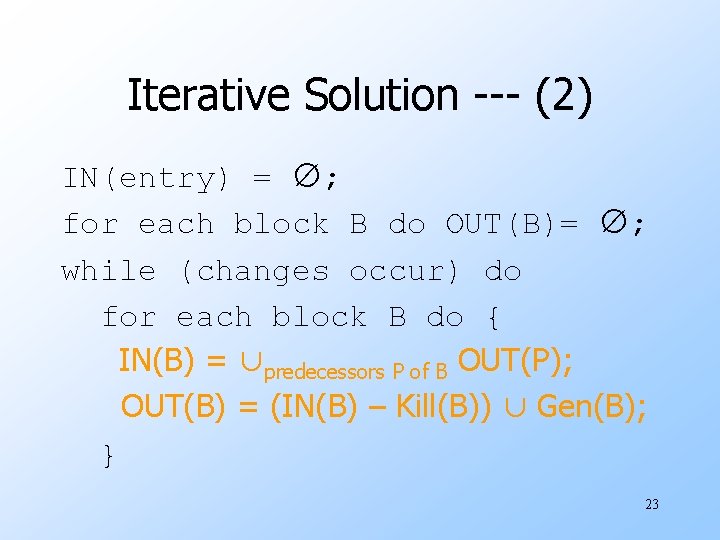
Iterative Solution --- (2) IN(entry) = ∅; for each block B do OUT(B)= ∅; while (changes occur) do for each block B do { IN(B) = ∪predecessors P of B OUT(P); OUT(B) = (IN(B) – Kill(B)) ∪ Gen(B); } 23

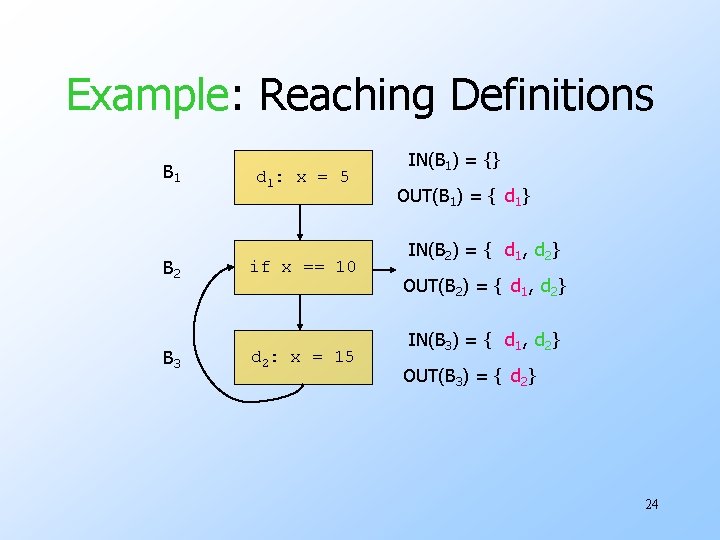
Example: Reaching Definitions B 1 B 2 B 3 d 1: x = 5 if x == 10 d 2: x = 15 IN(B 1) = {} OUT(B 1) = { d 1} IN(B 2) = { d 1, d 2} OUT(B 2) = { d 1, d 2} IN(B 3) = { d 1, d 2} OUT(B 3) = { d 2} 24

Aside: Notice the Conservatism u. Not only the most conservative assumption about when a def is killed or gen’d. u. Also the conservative assumption that any path in the flow graph can actually be taken. u. Fine, as long as the optimization is triggered by limitations on the set of RD’s, not by the assumption that a def does not reach. 25

Another Data-Flow Problem: Available Expressions u. An expression x+y is available at a point if no matter what path has been taken to that point from the entry, x+y has been evaluated, and neither x nor y have even possibly been redefined. u. Useful for global common-subexpression elimination. 26

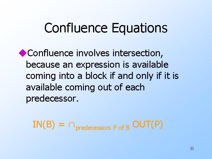
Equations for AE u. The equations for AE are essentially the same as for RD, with one exception. u. Confluence of paths involves intersection of sets of expressions rather than union of sets of definitions. 27

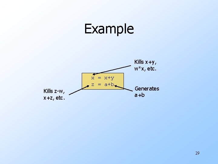
Gen(B) and Kill(B) u. An expression x+y is generated if it is computed in B, and afterwards there is no possibility that either x or y is redefined. u. An expression x+y is killed if it is not generated in B and either x or y is possibly redefined. 28

Example Kills x+y, w*x, etc. Kills z-w, x+z, etc. x = x+y z = a+b Generates a+b 29

Transfer Equations u. Transfer is the same idea: OUT(B) = (IN(B) – Kill(B)) ∪ Gen(B) 30

Confluence Equations u. Confluence involves intersection, because an expression is available coming into a block if and only if it is available coming out of each predecessor. IN(B) = ∩predecessors P of B OUT(P) 31

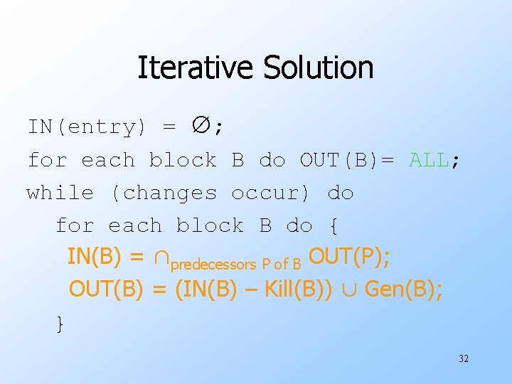
Iterative Solution IN(entry) = ∅; for each block B do OUT(B)= ALL; while (changes occur) do for each block B do { IN(B) = ∩predecessors P of B OUT(P); OUT(B) = (IN(B) – Kill(B)) ∪ Gen(B); } 32

Why It Works u An expression x+y is unavailable at point p iff there is a path from the entry to p that either: 1. Never evaluates x+y, or 2. Kills x+y after its last evaluation. u IN(entry) = ∅ takes care of (1). u OUT(B) = ALL, plus intersection during iteration handles (2). 33

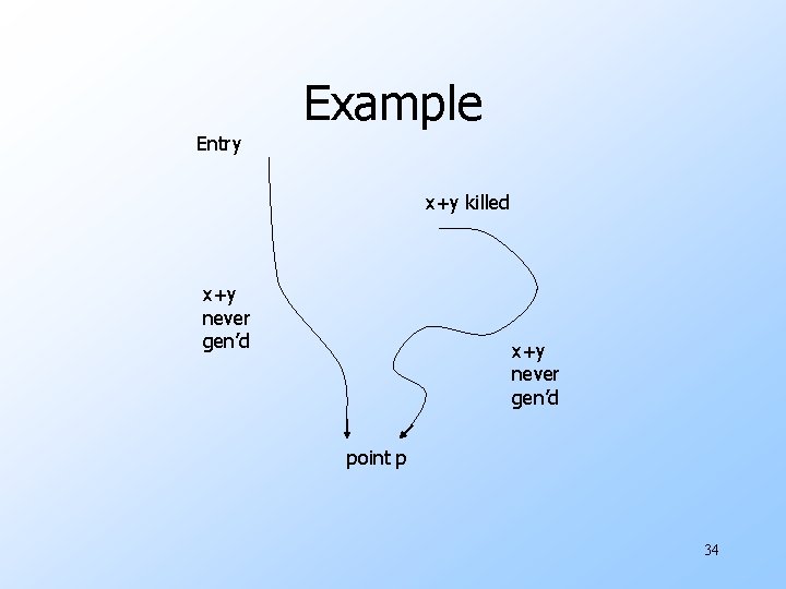
Example Entry x+y killed x+y never gen’d point p 34

Subtle Point u. It is conservative to assume an expression isn’t available, even if it is. u. But we don’t have to be “insanely conservative. ” w If after considering all paths, and assuming x+y killed by any possibility of redefinition, we still can’t find a path explaining its unavailability, then x+y is available. 35

Live Variable Analysis u. Variable x is live at a point p if on some path from p, x is used before it is redefined. u. Useful in code generation: if x is not live on exit from a block, there is no need to copy x from a register to memory. 36

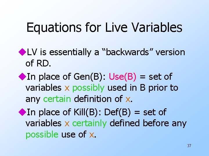
Equations for Live Variables u. LV is essentially a “backwards” version of RD. u. In place of Gen(B): Use(B) = set of variables x possibly used in B prior to any certain definition of x. u. In place of Kill(B): Def(B) = set of variables x certainly defined before any possible use of x. 37

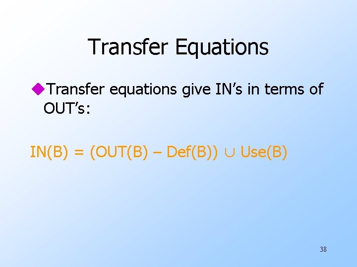
Transfer Equations u. Transfer equations give IN’s in terms of OUT’s: IN(B) = (OUT(B) – Def(B)) ∪ Use(B) 38

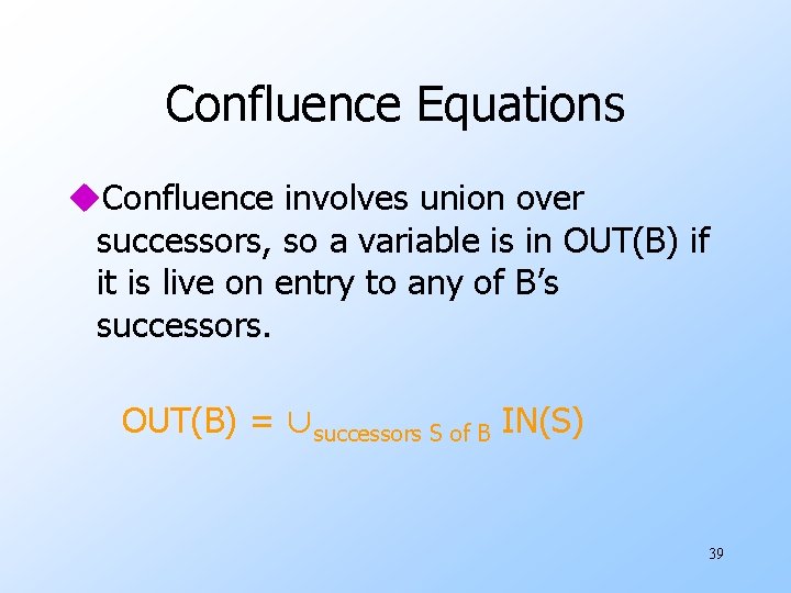
Confluence Equations u. Confluence involves union over successors, so a variable is in OUT(B) if it is live on entry to any of B’s successors. OUT(B) = ∪successors S of B IN(S) 39

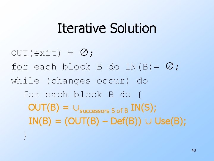
Iterative Solution OUT(exit) = ∅; for each block B do IN(B)= ∅; while (changes occur) do for each block B do { OUT(B) = ∪successors S of B IN(S); IN(B) = (OUT(B) – Def(B)) ∪ Use(B); } 40