DataFlow Analysis Chapter 8 Outline What is DataFlow

Data-Flow Analysis (Chapter 8)

Outline • • What is Data-Flow Analysis? Structure of an optimizing compiler An example: Reaching Definitions Basic Concepts: Lattices, Flow. Functions, and Fixed Points Taxonomy of Data-Flow Problems and Solutions Iterative Data-Flow Analysis Structural Data-Flow Analysis DU-Chains and SSA

Data-Flow Analysis • Input: A control flow graph • Output: A control flow graph with “global” information at every basic block Examples – Constant expressions: x+y*z – Live variables

Difficulties in Data-Flow Analysis • Input-dependent information • Undecidability of program analysis – Reachability of basic blocks – Arithmetic –. . .

Conservative data-flow analysis • Every piece of data-flow information sound • Every enabled optimization is correct • A superset of the execution sequences considered • In the reaching definition example superset of the reaching definitions computed is is a is

Iterative Computation of Reaching Definitions • Optimistically assume that at every block no definition is reached • Every basic block “generates” new definitions and “preserves” other definitions • No definition reaches ENTRY • Accumulate reaching definitions along different paths • Iteratively compute more and more definitions at every basic block • The process must terminate • The final solution is unique and conservative

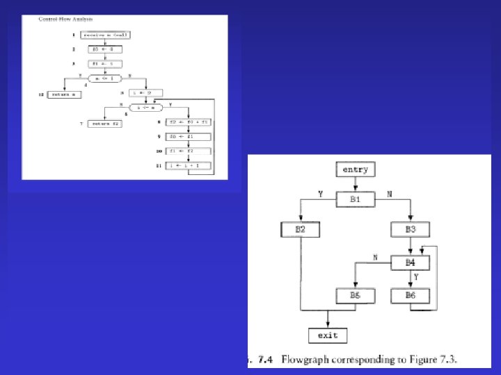
Generation Kill Preservation. V ector-8 bit Generation Vector – 8 bit B 1{1, 2, 3} {6, 7} {4, 5, 8} <00011001> <11100000> B 3{4} {8} {1, 2, 3, 5, 6, 7} <1110> <00010000> B 6{5, 6, 7, 8} {2, 3, 4} {1} <10000000> <00001111>

We define sets and corresponding bit vectors RCHout (i) that represent the definitions that reach the end of basic block i. as for RCHin(i), it is sufficient to initialize RCHout(i) by RCHout(i) = 0 or RCHout(i) = <0000> for all i. RCHout(i) = GEN(i) U (RCHin(i) ∩ PRSV(i))

To solve the system of bit vecto equations for RCHint(i) and RCHout(i), we simply initialize the RCHin(i) to the values given above and iterate application of the equations until no further changes result.

After iterating one more time, we have And iterating one more time produces no more changes so the above values are the solution. The rules for performing the iteration never change a 1 to a 0, they are monotone, so we guaranteed that the iteration process does terminate.

• The solution to the data flow equations gives us a global view of which definitions of varibales may reach which uses. • Ex. It shows that the definition of f 0 in basic block B 1 may reach the first use of f 0 in block B 6 and that along the execution path through basic block B 2, the variables i and f 2 are never defined. • We might use this information to optimize the program is to avoid allocation of storage for i and f 2 along the path through B 2.

Basic concepts: Lattices, Flow Functions and Fixed Points • A data flow analysis is performed by operating on elements of an algebraic structure called lattice. • It represent abstract properties of variables, expression, or other programming constructs for all possible executions of a procedure-independent of the values of the input data and usually independent of the control flow paths through procedure.

• We associate with each of the possible control flow and computational constructs in a procedure a so-called flow function that abstracts the effect of the constructor to its effect on the corresponding lattice elements. • In general, a Lattice L consists of a set of values and two operations called meet, denoted ⊓, and join denoted ⊔, that satisfy several properties, as follows:

• 1. for all x, y є L, there exist unique z and w є L such that x ⊓ y = z and x ⊔ y = w (closure) • 2. for all x, y є L, x ⊓ y = y ⊓ x and x ⊔ y = y ⊔ x. (commutatively). • 3. for x, y, z є L, (x ⊓ y) ⊓ z = x ⊓ (y ⊓ z) and (x ⊔ y) ⊔ z = x ⊔ (y ⊔ z) (associativity). • 4. There are two unique elements of L called bottom, denoted ⊥ and top, denoted ⊤ , such that for all x є L, x ⊓ ⊥ = ⊥ and x ⊔ ⊤ = ⊤ (existence of unique top and bottom elements).

• For x, y, z є L, • (x ⊓ y) ⊔ z = (x ⊔ z) ⊓ (y ⊔ z) and (x ⊔ y) ⊓ z = (x ⊓ z) ⊔ (y ⊓ z) (Distributive) • Most of the lattices we use have bit vectors as their elements and meet and join are bitwise AND and OR, respectively. • The bottom element of such a lattice is the bit vector of all zeroes and top is the vector of all ones. • We use BVn to denote the lattice of bit vectors of length n.

• Ex. The 8 -bit vector form a join lattice with <00101111> ⊔ <01100001> = <01101111>. • The join of two bit vector is the bit vector that has a one wherever either of them has a one and a zero • There are several ways to construct lattices by combining simple ones. – Product Operation : the product of two Lattices L 1 and L 2 with meet operators ⊓ 1 and ⊓ 2, respectively, which is written L 1 X L 2 , is {<x 1, x 2> | X 1 є L 1, x 2 є L 2} with meet operation as follows: – <x 1, x 2> ⊓ <y 1, y 2> = <x 1 ⊓ 1 y 1, x 2 ⊓ 2 y 2>

Dimensions for Data-Flow Problems • • The information provided “ralational” Vs. independent attributes The type of lattice and functions used The direction of information flow forward, backward, bidirectional

Example Data-Flow Problems • • Reaching Definitions Available Expressions Live Variables Upward Exposed Uses Copy-Propagation Analysis Constant-Propagation Analysis Partial-Redundency Analysis

Reaching Definitions • This determines which definition of a variable may reach use of the variable in a procedure. • It is a forward problem that uses a lattice of bit vectors with one bit corresponding to each definition of a variable

Available Expressions • Determines which expression are available at each point in a procedure. • It is a forward problem that uses a lattice of bit vectors in which a bit is assigned to each definition of an expression.

Live Variables • Determines for a given variable and a given point in a program where there is a use of the variable along some path from the point to the exit. • This is backward problem that uses bit vector in which each used of a variables is assigned a bit position.

Upward Exposed Uses • Determines what uses of variables at particular points are reached by particular definitions. • Definition of x in B 2 reaches the uses in B 4 and B 5, while the use in B 5 is reached by the definitions in B 2 and B 3

Copy-Propagation Analysis • Determines that on every path from a copy assignment, say x y, to a use of variable x there are no assignment to y. • This is a forward problem that uses bit vectors in which each bit position represents a copy assignment.

Constant-Propagation Analysis • Determines that on every path from an assignment of a constant to a variable, say, x const, to a use of x the only assignments to x assign it the value const.

Partial-Redundency Analysis • Determines what computations are performed twice (or more times) on some execution path without the operands being modified between the computation.

• The flow analysis problems listed above are not the only ones encountered in optimizations, but they are among the most important. • There are many approaches to solving data – flow problems, including the following:

Data-Flow Analysis Algorithms • • • Allen’s strongly connected regions Kildall’s iterative algorithm Ullman’s T 1 -T 2 analysis Kennedy’s node-listing algorithm Farrow, Kennedy, and Zuconi’s graph grammar approach • Rosen’s high-level approach • structural analysis • slotwise analysis

We will concentrate on three approaches: 1. The simple iterative approach with several strategies for determining the order of the iterations. 2. An elimination or control-tree-based method using intervals 3. Another control-tree based method using structural analysis.

Iterative analysis: • It is the method which we have used in the example of Fibonacci series. • It is easy to implement and as a result, it is frequently used. • Due to Iterative method of forward analysis, we can easily generalize methods for backward and bidirectional analysis.

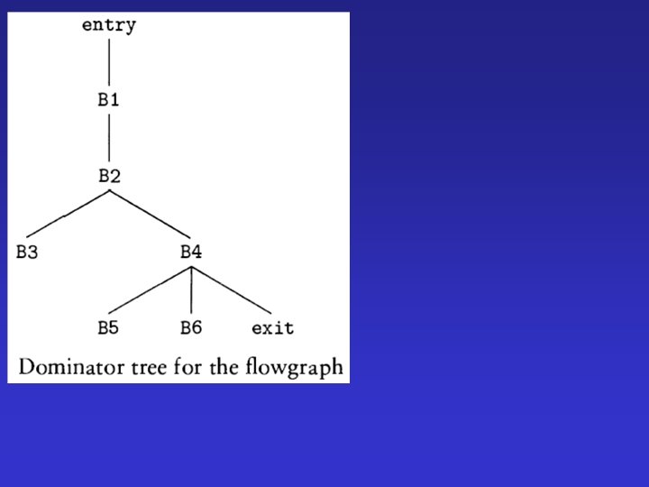
Control-tree-based data flow analysis: • The algorithms for control-tree-based data-flow analysis namely, interval analysis and structural analysis are very similar to the control tree based structural analysis studied in chapter 7 • Slightly harder to the iterative analysis

Structural Data-Flow Analysis • Phase 1: Compute “the effect” of every program construct in a bottom-up fashion on the tree of control flow constructs (control-tree) • Phase 2: Propagates the data-flow value in a top-down fashion into basic blocks • (This part is covered in the chapeter 7 while discussing the loop structures)

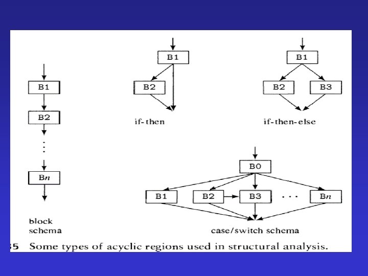
Handling Arbitrary CFGs • Need to handle arbitrary acyclic regions • Need to to handle irreducible components (improper regions)

Handling Arbitrary CFGs • Need to handle arbitrary acyclic regions • Need to handle arbitrary cyclic regions – Reducible regions – irreducible components (improper regions)

Handling Improper Regions • • Ignore Node splitting Solve iteratively for every initial value Solve iteratively over LF

Structural Backward Analysis • Tricky • For constructs with single exit “reverse” equation direction • For acyclic constructs with multiple exits use join • For cyclic reducible constructs with multiple exits--- break the cycle and use join • Cyclic improper regions are handled like the forward case

Bottom-Up Phase Backward Problems (if-then) Fif/Y then Fthen if Fif-then=(F if/Y° Fthen) Fif/N if-then Fif-then

Top-Down Phase Backward Problems (if-then) out(then)= out(if-then) Fif/Y then Fthen if out(if) = Fthen(out(then)) out(if-then) Fif/N if-then Fif-then

Implementation • Represent the computation of canonic cases with functions (if-then-else, while) • Use graphs to represent arbitrary functional computations

Automatic Construction of Data-Flow Analyzers • Not commonly used so far • Kildall developed a tool for iterative data flow analysis (1973) • The PAG (1995) system allows systematic construction of iterative data-flow analysis • The Sharlit (1992) system generates noniterative data-flow analyzers – Finds regular “path-expressions” in CFG – Convert into effect functions

Def-Use, Use-Def Chains • Sparse data-flow information on flow of variables between assignments • Can be used to improve the efficiency of iterative dataflow analysis • A du-chain for a variable v connects a definition of v to all the uses of this definition • A ud-chain for a variable v connects a use of v to all the definitions that may flow to it • A web for a variable v is the maximal union of interesting du-chains for v

entry z>1 Y N x 2 x 1 z>2 N Y z x-3 x 4 y x+1 z x+7 exit

Static Single Assignment (SSA) • A normal form of the program such that defuse is immediate • A separate variable for every assignment • A function combines the values of relevant variables • Simplifies some optimizations • Increases program’s size

entry z 1>1 Y N x 2 2 x 1 1 z 1>2 N Y x 3 (x 1, x 2) ; z 2 x 3 -3 x 4 4 y 1 x 1+1 z 3 x 4+7 exit

Flow graph to be translated to minimal SSA form The iterative characterization of dominance frontiers given , computer for variable k: DF 1 ({entry, B 1, B 3}) = {B 2} DF 2 ({entry, B 1, B 3}) = DF({entry, B 1, B 2, B 3}) = B 2

For variable i: DF 1 ({entry, B 1, B 3, B 6}) = {B 2, exit} DF 2 ({entry, B 1, B 3, B 6}) = DF({entry, B 1, B 2, B 3, B 6, exit}) For variable j: DF 1({entry, B 1, B 3}) = {B 2} DF 2({entry, B 1, B 3}) = DF ({entry, B 1, B 2, B 3}) = {B 2}

B 2 requires a function for each of i, j and k and exit needs one for i

Handling Pointers and Arrays • • Complicated!!! Treated conservatively in most compilers The frontier of research A simple “reduction” x a[i] x access(a, i) a update(a, i, 4) a[i] 4 • Direct solutions yield more precise solutions

More Ambitious Data-Flow Analysis • Data-Flow analysis can yield “interesting” information on program behavior • Signs of variables • Non-trivial constant values • Termination properties • Complicated bugs • Partial correctness

int f(int x) { if (x > 100) return x -10; else return f(f(x+11)); } void main() { scanf(“%d”, &x); if (x > 100) printf(“%dn”, 91); else printf(“%dn”, f(x)); }