Data Analysis Peter Fox Data Science ITECCSCIERTH43506350 Week

Data Analysis Peter Fox Data Science – ITEC/CSCI/ERTH-4350/6350 Week 5, September 24, 2013 1

Contents • Preparing for data analysis, completing and presenting results • Statistics, distributions, filtering, etc. • Errors and some uncertainty… • Visualization as an information tool and analysis tool • New visualization methods (new types of data) • Use, citation, attribution and reproducability 2

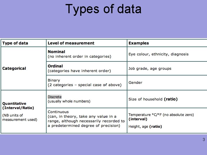
Types of data 3

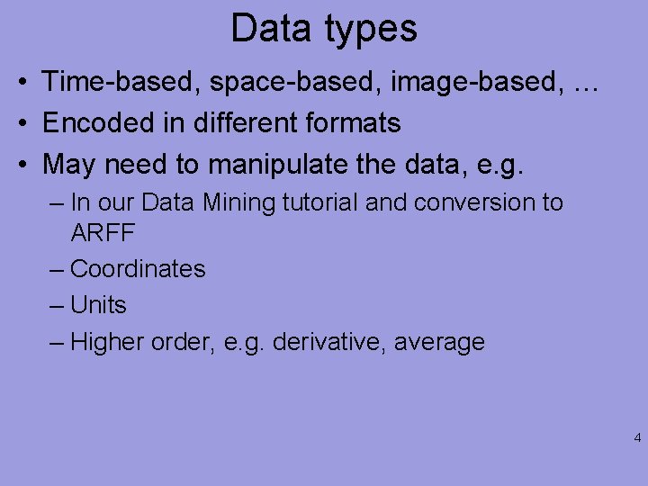
Data types • Time-based, space-based, image-based, … • Encoded in different formats • May need to manipulate the data, e. g. – In our Data Mining tutorial and conversion to ARFF – Coordinates – Units – Higher order, e. g. derivative, average 4

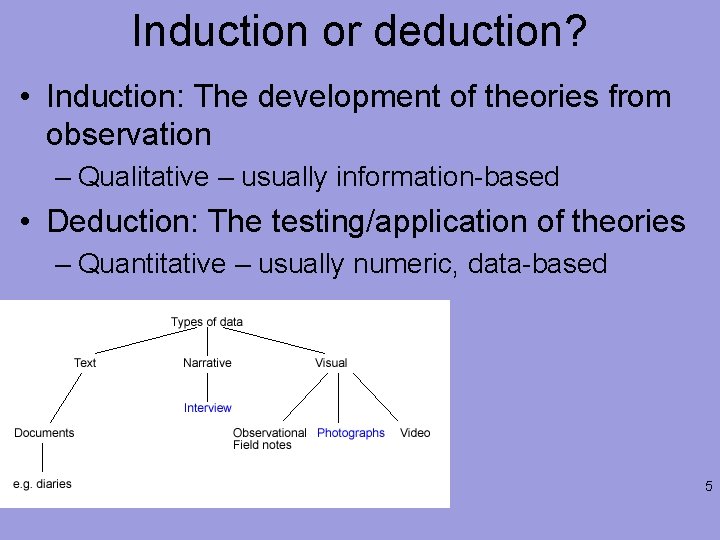
Induction or deduction? • Induction: The development of theories from observation – Qualitative – usually information-based • Deduction: The testing/application of theories – Quantitative – usually numeric, data-based 5

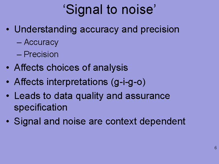
‘Signal to noise’ • Understanding accuracy and precision – Accuracy – Precision • Affects choices of analysis • Affects interpretations (g-i-g-o) • Leads to data quality and assurance specification • Signal and noise are context dependent 6

Other considerations • Continuous or discrete • Underlying reference system • Oh yeah: metadata standards and conventions • The underlying data structures are important at this stage but there is a tendency to read in partial data – Why is this a problem? – How to ameliorate any problems? 7

Outlier • An extreme, or atypical, data value(s) in a sample. • They should be considered carefully, before exclusion from analysis. • For example, data values maybe recorded erroneously, and hence they may be corrected. • However, in other cases they may just be surprisingly different, but not necessarily 'wrong'. 8

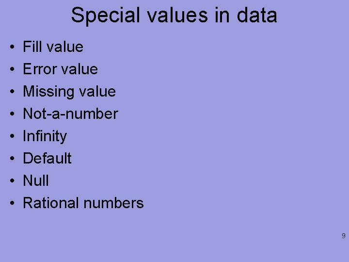
Special values in data • • Fill value Error value Missing value Not-a-number Infinity Default Null Rational numbers 9

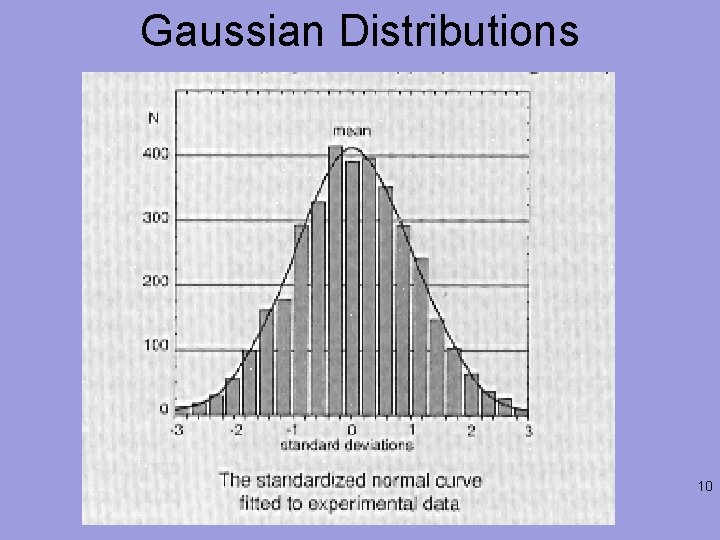
Gaussian Distributions 10

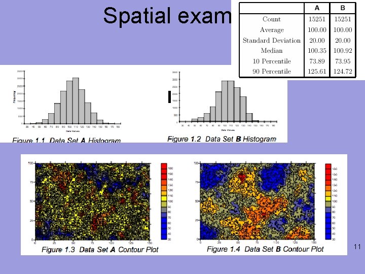
Spatial example 11

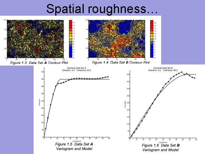
Spatial roughness… 12

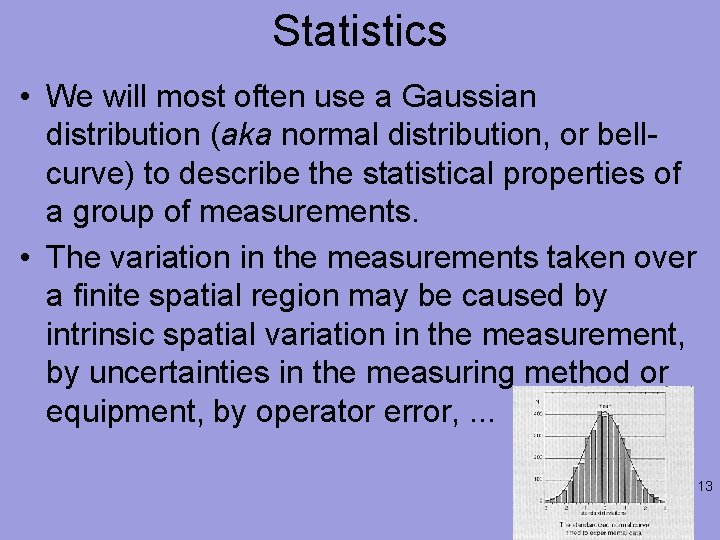
Statistics • We will most often use a Gaussian distribution (aka normal distribution, or bellcurve) to describe the statistical properties of a group of measurements. • The variation in the measurements taken over a finite spatial region may be caused by intrinsic spatial variation in the measurement, by uncertainties in the measuring method or equipment, by operator error, . . . 13

Mean and standard deviation • The mean, m, of n values of the measurement of a property z (the average). – m = [ SUM {i=1, n} zi ] / n • The standard deviation s of the measurements is an indication of the amount of spread in the measurements with respect to the mean. – s 2 = [ SUM {i=1, n} ( zi - m )2 ] /n • The quantity s 2 is known as the variance of the measurements. 14

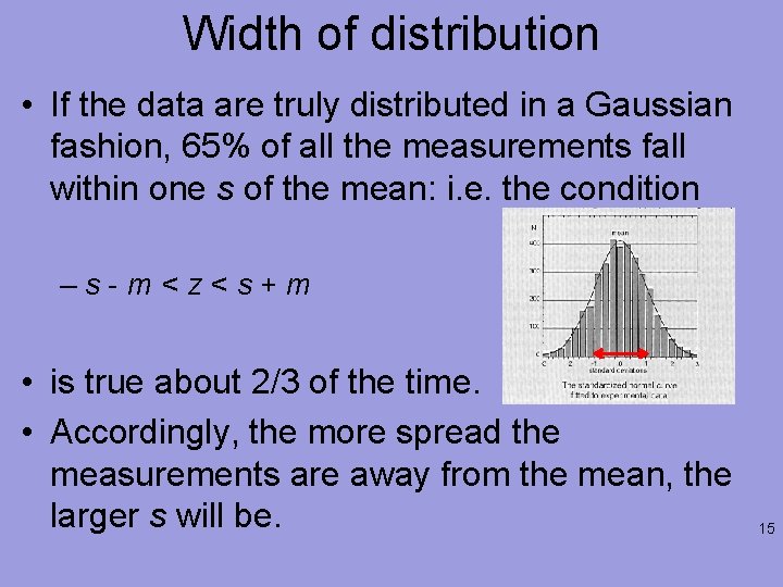
Width of distribution • If the data are truly distributed in a Gaussian fashion, 65% of all the measurements fall within one s of the mean: i. e. the condition –s-m<z<s+m • is true about 2/3 of the time. • Accordingly, the more spread the measurements are away from the mean, the larger s will be. 15

Measurement description – by its mean and standard deviation. • Often a measurement at a sampling point is made several times and these measurements are grouped into a single one, giving the statistics. • If only a single measurement is made (due to cost or time), then we need to estimate the standard deviation in some way, perhaps by the known characteristics of our measuring device. • An estimate of the standard deviation of a measurement is more important than the measurement itself. 16

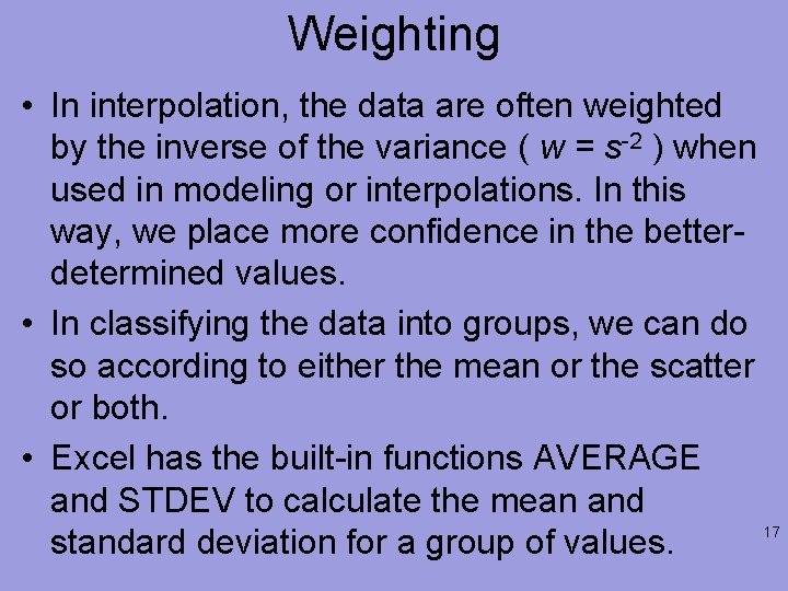
Weighting • In interpolation, the data are often weighted by the inverse of the variance ( w = s-2 ) when used in modeling or interpolations. In this way, we place more confidence in the betterdetermined values. • In classifying the data into groups, we can do so according to either the mean or the scatter or both. • Excel has the built-in functions AVERAGE and STDEV to calculate the mean and 17 standard deviation for a group of values.

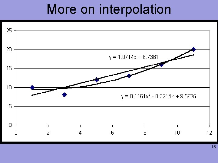
More on interpolation 18

Global/ Local Methods • Global methods ~ in which all the known data are considered • Local methods ~ in which only nearby data are used. • Local methods and most often the global methods also rely on the premise that nearby points are more similar than distant points. • Inverse Distance Weighting (IDW) is an example of a global method. 19

More… • Local methods include bilinear interpolation and planar interpolation within triangles delineated by 3 known points. • Global Surface Trends: Fitting some form of a polynomial to data to predict values at unsampled points. • Such fitting is done by regression – estimates of coefficients by least-squares fit to data. – Produces a continuous field – Continuous first derivatives – Values NOT reproduced exactly at observation points 20

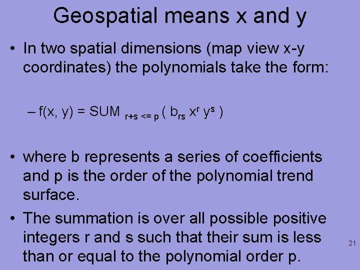
Geospatial means x and y • In two spatial dimensions (map view x-y coordinates) the polynomials take the form: – f(x, y) = SUM r+s <= p ( brs xr ys ) • where b represents a series of coefficients and p is the order of the polynomial trend surface. • The summation is over all possible positive integers r and s such that their sum is less than or equal to the polynomial order p. 21

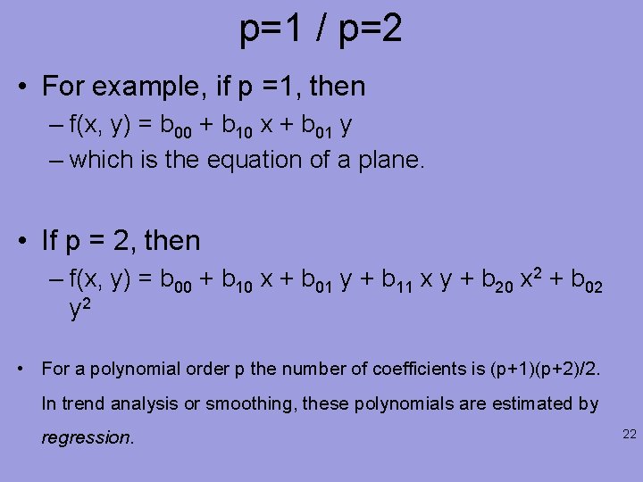
p=1 / p=2 • For example, if p =1, then – f(x, y) = b 00 + b 10 x + b 01 y – which is the equation of a plane. • If p = 2, then – f(x, y) = b 00 + b 10 x + b 01 y + b 11 x y + b 20 x 2 + b 02 y 2 • For a polynomial order p the number of coefficients is (p+1)(p+2)/2. In trend analysis or smoothing, these polynomials are estimated by regression. 22

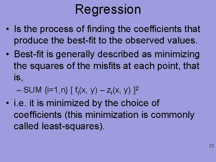
Regression • Is the process of finding the coefficients that produce the best-fit to the observed values. • Best-fit is generally described as minimizing the squares of the misfits at each point, that is, – SUM {i=1, n} [ fi(x, y) – zi(x, y) ]2 • i. e. it is minimized by the choice of coefficients (this minimization is commonly called least-squares). 23

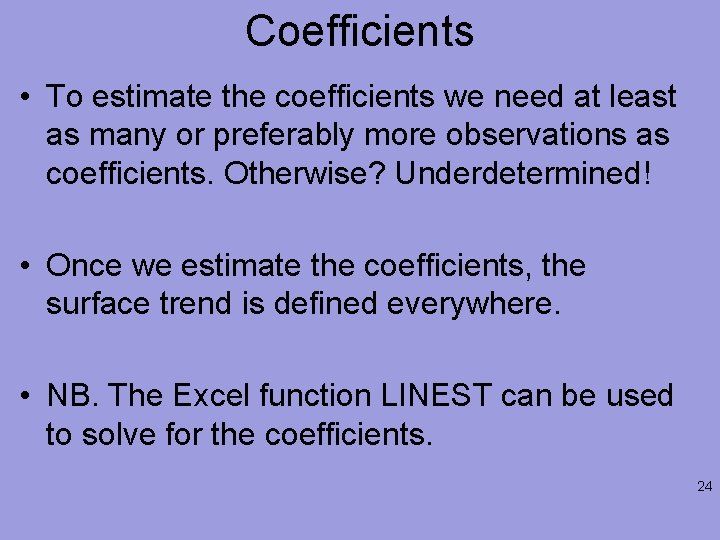
Coefficients • To estimate the coefficients we need at least as many or preferably more observations as coefficients. Otherwise? Underdetermined! • Once we estimate the coefficients, the surface trend is defined everywhere. • NB. The Excel function LINEST can be used to solve for the coefficients. 24

Choices… • The choice of how many coefficients to use (the order of the polynomial) depends on how smooth you think the variations in the property is, and on how well the data are fit by lower order polynomials. • In general, adding coefficients always improves the fit to the data to the extreme that if the number of coefficients equals the number of observations, the data can be fit perfectly. 25 • But this assumes that the data are perfect.

Multi-variate analysis • Multivariate analysis is the procedure to use if we want to see if there is a correlation between any pair of attributes in our data. • As earlier, you perform a linear regression to find the correlations. 26

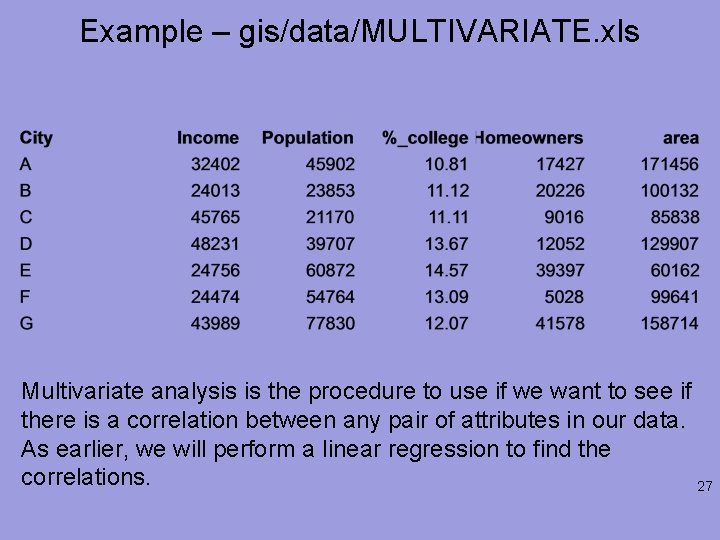
Example – gis/data/MULTIVARIATE. xls Multivariate analysis is the procedure to use if we want to see if there is a correlation between any pair of attributes in our data. As earlier, we will perform a linear regression to find the correlations. 27

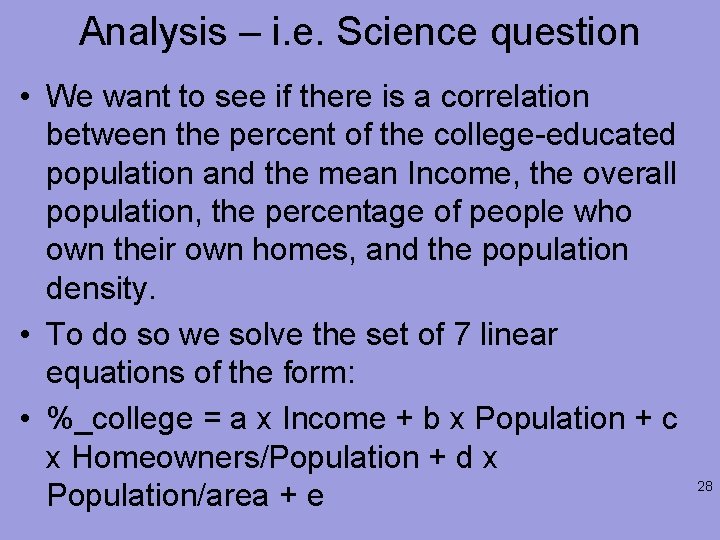
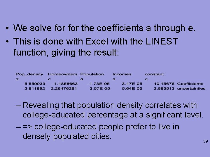
Analysis – i. e. Science question • We want to see if there is a correlation between the percent of the college-educated population and the mean Income, the overall population, the percentage of people who own their own homes, and the population density. • To do so we solve the set of 7 linear equations of the form: • %_college = a x Income + b x Population + c x Homeowners/Population + d x Population/area + e 28

• We solve for the coefficients a through e. • This is done with Excel with the LINEST function, giving the result: – Revealing that population density correlates with college-educated percentage at a significant level. – => college-educated people prefer to live in densely populated cities. 29

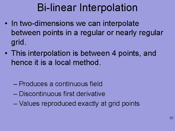
Bi-linear Interpolation • In two-dimensions we can interpolate between points in a regular or nearly regular grid. • This interpolation is between 4 points, and hence it is a local method. – Produces a continuous field – Discontinuous first derivative – Values reproduced exactly at grid points 30

Example x 0, y 0 t = [ x 0 – x 1 ] / [ x 2 - x 1 ] and u = [ y 0 – y 1 ] / [ y 4 - y 1 ] • The red squares represent 4 known values of z(x, y) and our goal is to estimate the value of z at the new point (blue circle) at (x 0, y 0). 31

Calculating… • Let • t = [ x 0 – x 1 ] / [ x 2 - x 1 ] and • u = [ y 0 – y 1 ] / [ y 4 - y 1 ] i. e. the fractional distances the new point is along the grid axes in x and y, respectively, where the subscripts refer to the known points as numbered above. Then • z (x 0 , y 0 ) = (1 -t) (1 -u) z 1 + t (1 -u) z 2 + t u z 3 + (1 -t ) u z 4 32

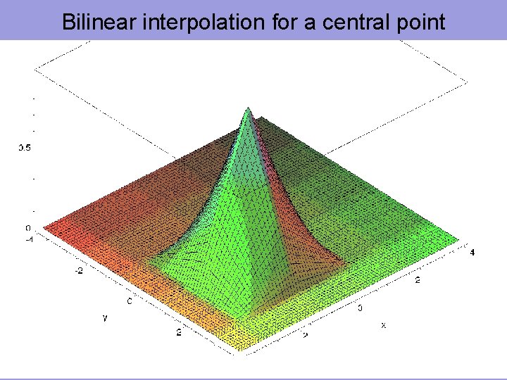
Bilinear interpolation for a central point 33

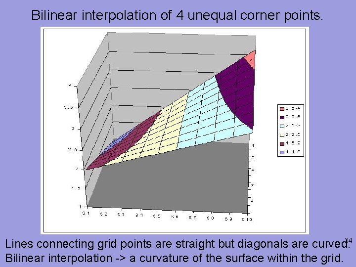
Bilinear interpolation of 4 unequal corner points. 34 Lines connecting grid points are straight but diagonals are curved. Bilinear interpolation -> a curvature of the surface within the grid.

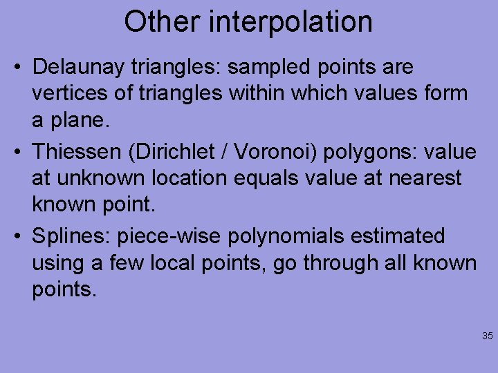
Other interpolation • Delaunay triangles: sampled points are vertices of triangles within which values form a plane. • Thiessen (Dirichlet / Voronoi) polygons: value at unknown location equals value at nearest known point. • Splines: piece-wise polynomials estimated using a few local points, go through all known points. 35

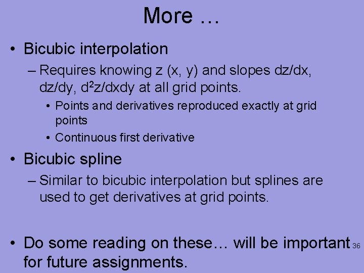
More … • Bicubic interpolation – Requires knowing z (x, y) and slopes dz/dx, dz/dy, d 2 z/dxdy at all grid points. • Points and derivatives reproduced exactly at grid points • Continuous first derivative • Bicubic spline – Similar to bicubic interpolation but splines are used to get derivatives at grid points. • Do some reading on these… will be important 36 for future assignments.

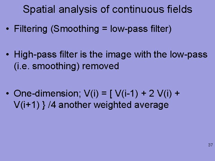
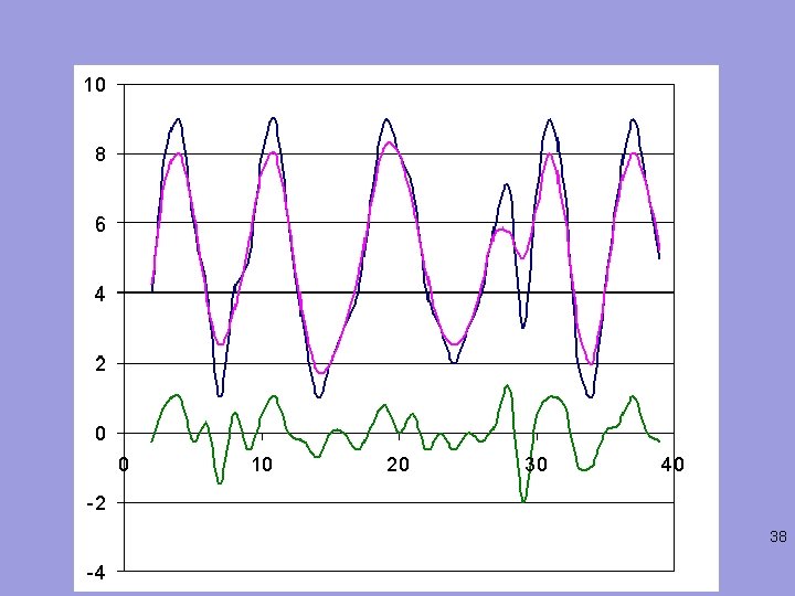
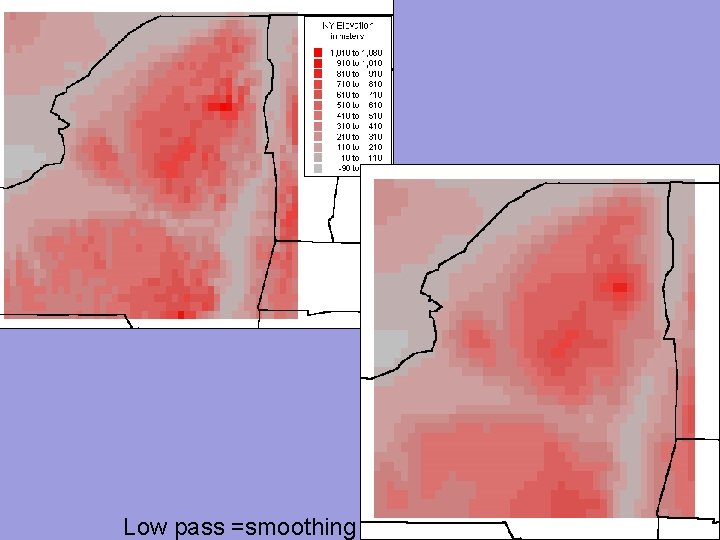
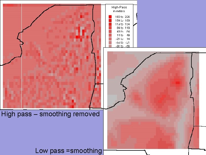
Spatial analysis of continuous fields • Filtering (Smoothing = low-pass filter) • High-pass filter is the image with the low-pass (i. e. smoothing) removed • One-dimension; V(i) = [ V(i-1) + 2 V(i) + V(i+1) } /4 another weighted average 37

38

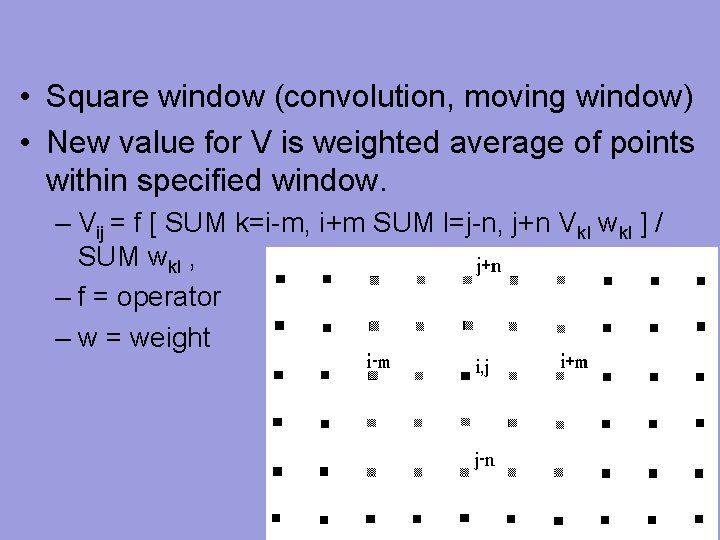
• Square window (convolution, moving window) • New value for V is weighted average of points within specified window. – Vij = f [ SUM k=i-m, i+m SUM l=j-n, j+n Vkl wkl ] / SUM wkl , – f = operator – w = weight 39

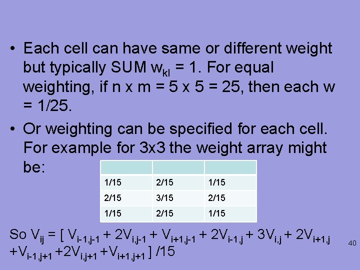
• Each cell can have same or different weight but typically SUM wkl = 1. For equal weighting, if n x m = 5 x 5 = 25, then each w = 1/25. • Or weighting can be specified for each cell. For example for 3 x 3 the weight array might be: 1/15 2/15 3/15 2/15 1/15 So Vij = [ Vi-1, j-1 + 2 Vi, j-1 + Vi+1, j-1 + 2 Vi-1, j + 3 Vi, j + 2 Vi+1, j +Vi-1, j+1 +2 Vi, j+1 +Vi+1, j+1 ] /15 40

41 Low pass =smoothing

High pass – smoothing removed 42 Low pass =smoothing

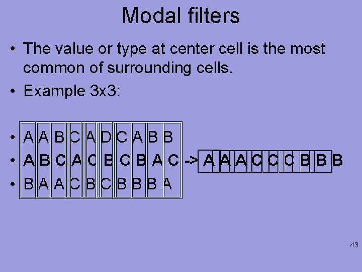
Modal filters • The value or type at center cell is the most common of surrounding cells. • Example 3 x 3: • A A B C A D C A B B • A B C A C B A C -> A A A C C C B B B • B A A C B B B A 43

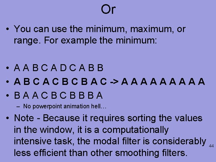
Or • You can use the minimum, maximum, or range. For example the minimum: • A A B C A D C A B B • A B C A C B A C -> A A A A A • B A A C B B B A – No powerpoint animation hell… • Note - Because it requires sorting the values in the window, it is a computationally intensive task, the modal filter is considerably 44 less efficient than other smoothing filters.

Median filter • Median filters can be used to emphasize the longerrange variability in an image, effectively acting to smooth the image. • This can be useful for reducing the noise in an image. The algorithm operates by calculating the median value (middle value in a sorted list) in a moving window centered on each grid cell. • The median value is not influenced by anomalously high or low values in the distribution to the extent that the average is. • As such, the median filter is far less sensitive to shot 45 noise in an image than the mean filter.

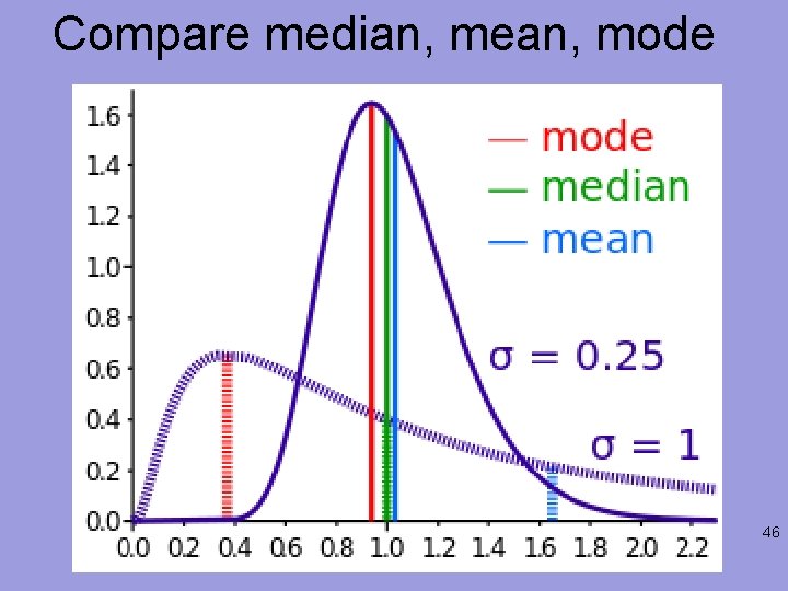
Compare median, mean, mode 46

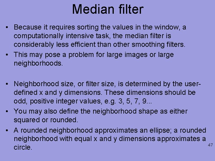
Median filter • Because it requires sorting the values in the window, a computationally intensive task, the median filter is considerably less efficient than other smoothing filters. • This may pose a problem for large images or large neighborhoods. • Neighborhood size, or filter size, is determined by the userdefined x and y dimensions. These dimensions should be odd, positive integer values, e. g. 3, 5, 7, 9. . . • You may also define the neighborhood shape as either squared or rounded. • A rounded neighborhood approximates an ellipse; a rounded neighborhood with equal x and y dimensions approximates a 47 circle.

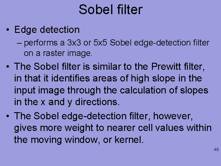
Sobel filter • Edge detection – performs a 3 x 3 or 5 x 5 Sobel edge-detection filter on a raster image. • The Sobel filter is similar to the Prewitt filter, in that it identifies areas of high slope in the input image through the calculation of slopes in the x and y directions. • The Sobel edge-detection filter, however, gives more weight to nearer cell values within the moving window, or kernel. 48

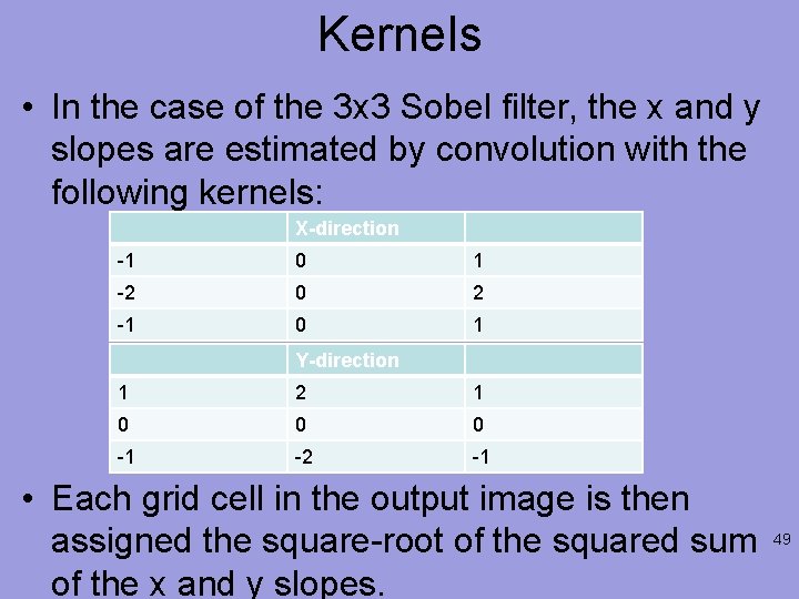
Kernels • In the case of the 3 x 3 Sobel filter, the x and y slopes are estimated by convolution with the following kernels: X-direction -1 0 1 -2 0 2 -1 0 1 Y-direction 1 2 1 0 0 0 -1 -2 -1 • Each grid cell in the output image is then assigned the square-root of the squared sum 49 of the x and y slopes.

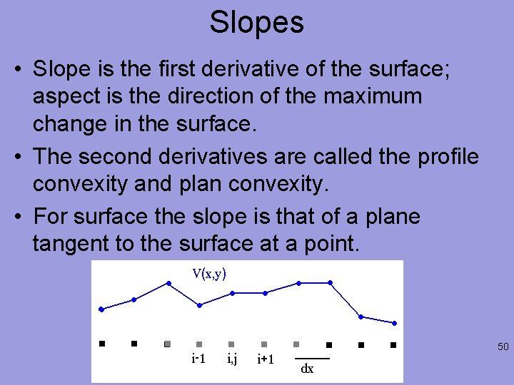
Slopes • Slope is the first derivative of the surface; aspect is the direction of the maximum change in the surface. • The second derivatives are called the profile convexity and plan convexity. • For surface the slope is that of a plane tangent to the surface at a point. 50

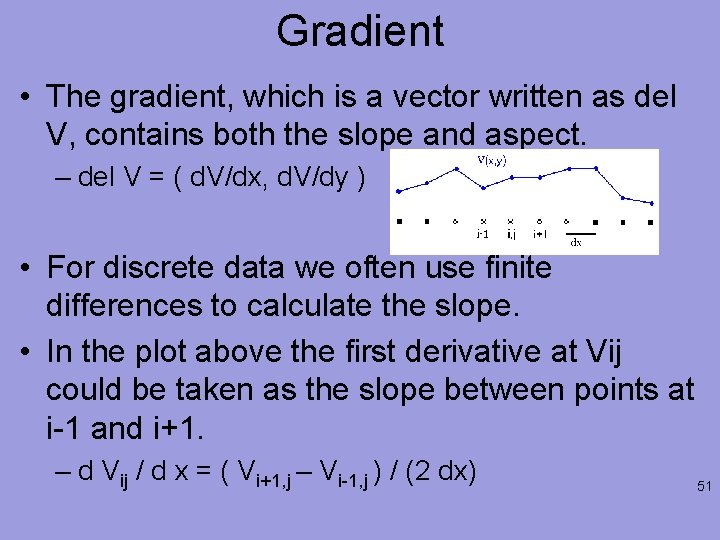
Gradient • The gradient, which is a vector written as del V, contains both the slope and aspect. – del V = ( d. V/dx, d. V/dy ) • For discrete data we often use finite differences to calculate the slope. • In the plot above the first derivative at Vij could be taken as the slope between points at i-1 and i+1. – d Vij / d x = ( Vi+1, j – Vi-1, j ) / (2 dx) 51

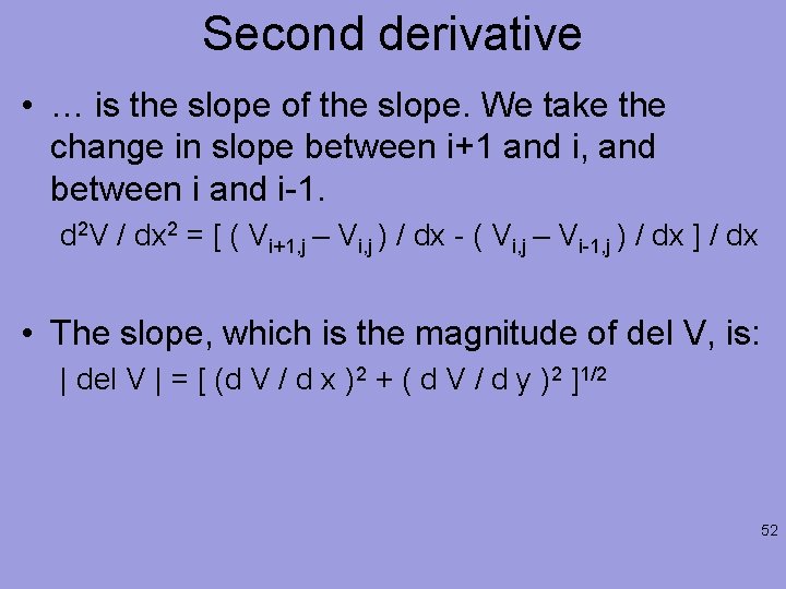
Second derivative • … is the slope of the slope. We take the change in slope between i+1 and i, and between i and i-1. d 2 V / dx 2 = [ ( Vi+1, j – Vi, j ) / dx - ( Vi, j – Vi-1, j ) / dx ] / dx • The slope, which is the magnitude of del V, is: | del V | = [ (d V / d x )2 + ( d V / d y )2 ]1/2 52

Errors • Personal errors are mistakes on the part of the experimenter. It is your responsibility to make sure that there are no errors in recording data or performing calculations • Systematic errors tend to decrease or increase all measurements of a quantity, (for instance all of the measurements are too large). E. g. calibration • Random errors are also known as statistical uncertainties, and are a series of small, unknown, and uncontrollable events 53

Errors • Statistical uncertainties are much easier to assign, because there are rules for estimating the size • E. g. If you are reading a ruler, the statistical uncertainty is half of the smallest division on the ruler. Even if you are recording a digital readout, the uncertainty is half of the smallest place given. This type of error should always be recorded for any measurement 54

Standard measures of error • Absolute deviation – is simply the difference between an experimentally determined value and the accepted value • Relative deviation – is a more meaningful value than the absolute deviation because it accounts for the relative size of the error. The relative percentage deviation is given by the absolute deviation divided by the accepted value and multiplied by 100% • Standard deviation – standard definition 55

Standard deviation • the average value is found by summing and dividing by the number of determinations. Then the residuals are found by finding the absolute value of the difference between each determination and the average value. Third, square the residuals and sum them. Last, divide the result by the number of determinations - 1 and take the square root. 56

Spatial analysis of continuous fields • Possibly more important than our answer is our confidence in the answer. • Our confidence is quantified by uncertainties as discussed earlier. • Once we combine numbers, we need to be able to assess how the uncertainties change for the combination. • This is called propagation of errors or more correctly the propagation of our understanding/ estimate of errors in the result 57 we are looking at…

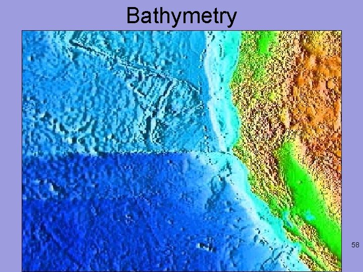
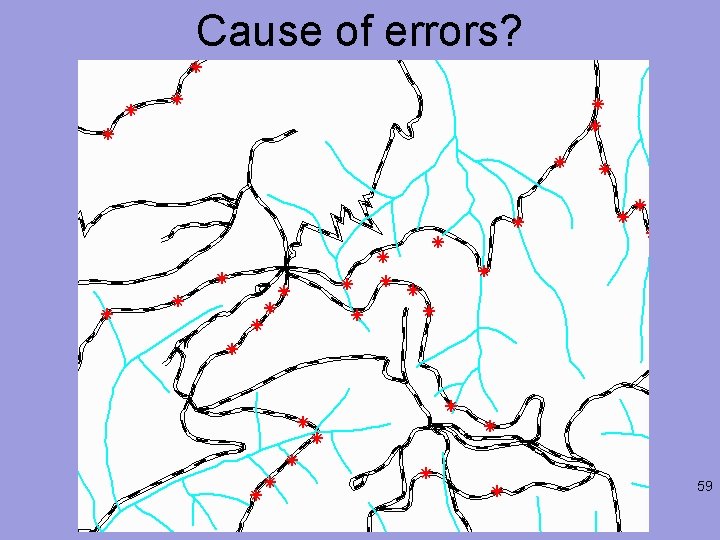
Bathymetry 58

Cause of errors? 59

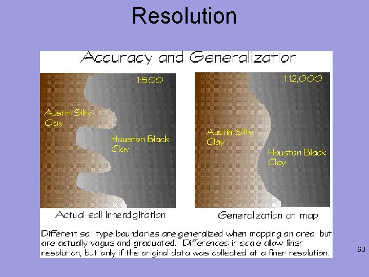
Resolution 60

Reliability • Changes in data over time • Non-uniform coverage • Map scales • Observation density • Sampling theorem (aliasing) • Surrogate data and their relevance • Round-off errors in computers 61

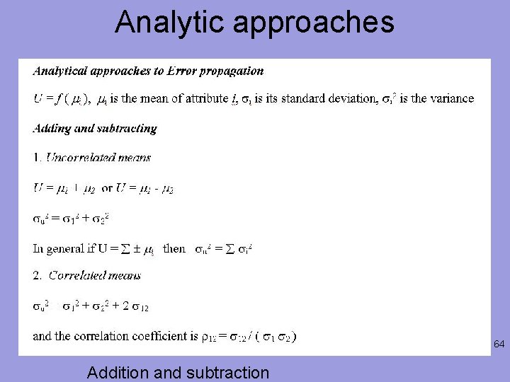
Propagating errors • This is an unfortunate term – it means making sure that the result of the analysis carries with it a calculation (rather than an estimate) of the error • E. g. if C=A+B (your analysis), then ∂C=∂A+∂B • E. g. if C=A-B (your analysis), then ∂C=∂A+∂B! • Exercise – it’s not as simple for other calcs. • When the function is not merely addition, subtraction, multiplication, or division, the error propagation must be defined by the total 62 derivative of the function.

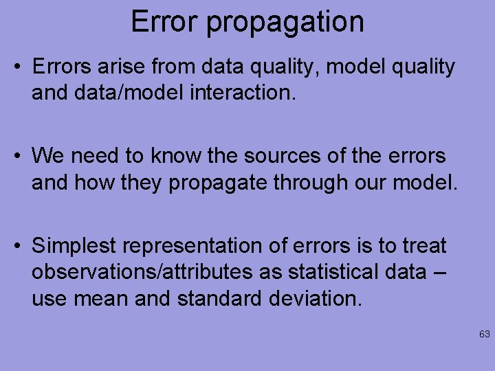
Error propagation • Errors arise from data quality, model quality and data/model interaction. • We need to know the sources of the errors and how they propagate through our model. • Simplest representation of errors is to treat observations/attributes as statistical data – use mean and standard deviation. 63

Analytic approaches 64 Addition and subtraction

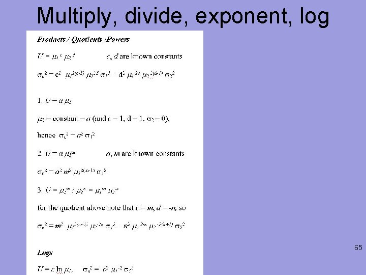
Multiply, divide, exponent, log 65

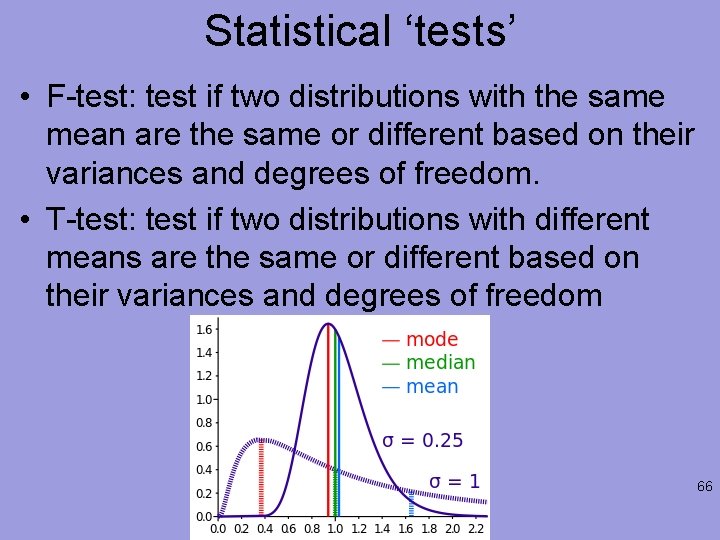
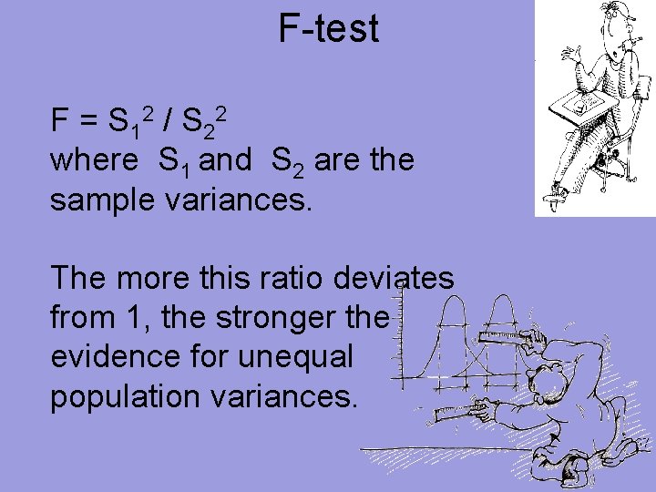
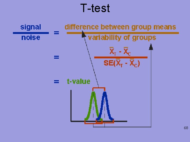
Statistical ‘tests’ • F-test: test if two distributions with the same mean are the same or different based on their variances and degrees of freedom. • T-test: test if two distributions with different means are the same or different based on their variances and degrees of freedom 66

F-test F = S 12 / S 22 where S 1 and S 2 are the sample variances. The more this ratio deviates from 1, the stronger the evidence for unequal population variances. 67

T-test 68

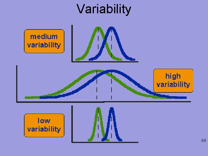
Variability 69

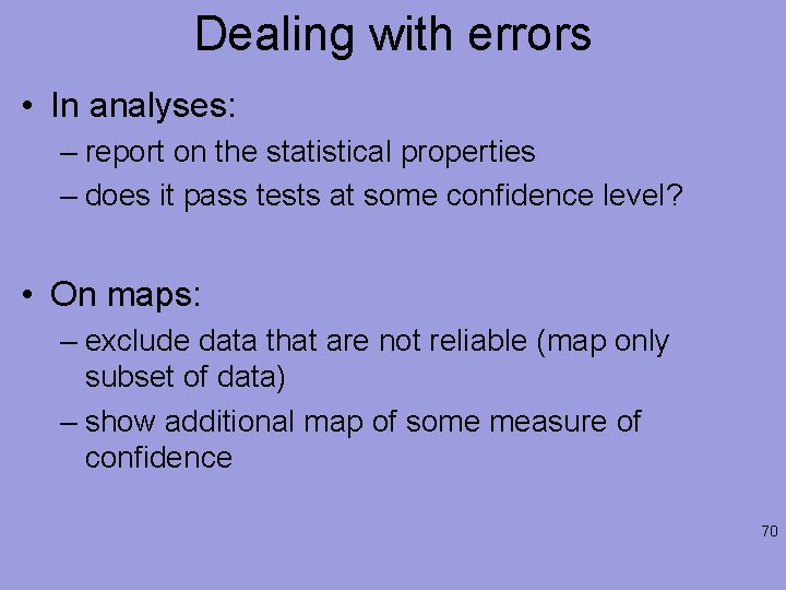
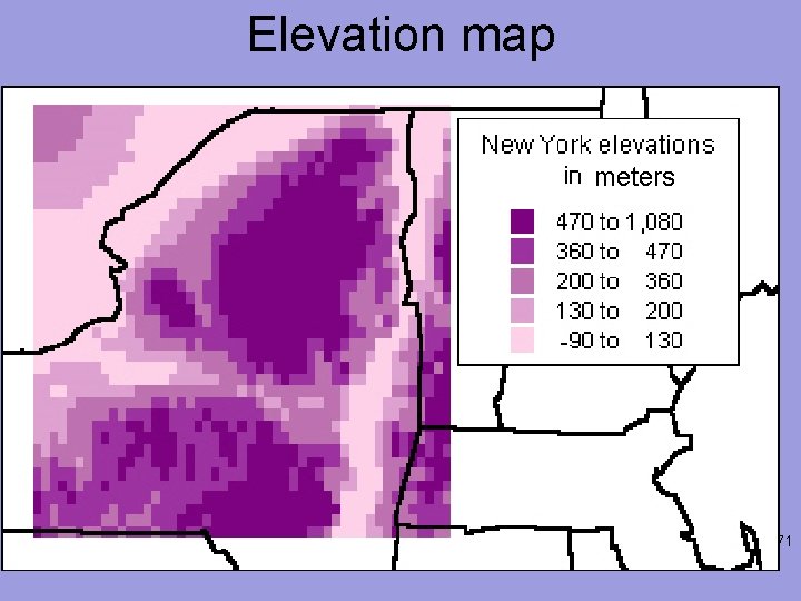
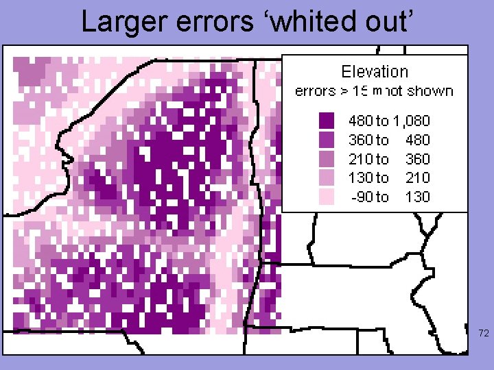
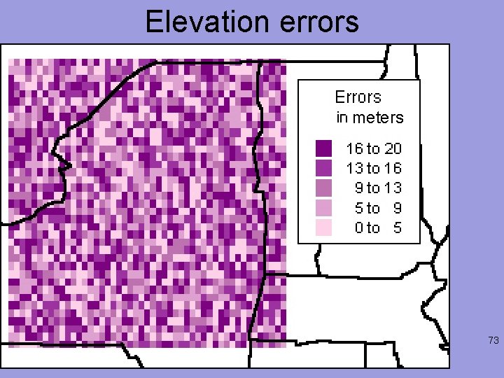
Dealing with errors • In analyses: – report on the statistical properties – does it pass tests at some confidence level? • On maps: – exclude data that are not reliable (map only subset of data) – show additional map of some measure of confidence 70

Elevation map meters 71

Larger errors ‘whited out’ m 72

Elevation errors meters 73

Types of analysis • • Preliminary Detailed Summary Reporting the results and propagating uncertainty • Qualitative v. quantitative, e. g. see http: //hsc. uwe. ac. uk/dataanalysis/index. asp 74

What is preliminary analysis? • Self-explanatory…? • Down sampling…? • The more measurements that can be made of a quantity, the better the result – Reproducibility is an axiom of science • When time is involved, e. g. a signal – the ‘sampling theorem’ – having an idea of the hypothesis is useful, e. g. periodic versus aperiodic or other… • http: //en. wikipedia. org/wiki/Nyquist– Shannon_sampling_theorem 75

Detailed analysis • Most important distinction between initial and the main analysis is that during initial data analysis it refrains from any analysis. • Basic statistics of important variables – Scatter plots – Correlations – Cross-tabulations • Dealing with quality, bias, uncertainty, accuracy, precision limitations - assessing • Dealing with under- or over-sampling • Filtering, cleaning 76

Summary analysis • Collecting the results and accompanying documentation • Repeating the analysis (yes, it’s obvious) • Repeating with a subset • Assessing significance, e. g. the confusion matrix we used in the supervised classification example for data mining, pvalues (null hypothesis probability) 77

Reporting results/ uncertainty • Consider the number of significant digits in the result which is indicative of the certainty of the result • Number of significant digits depends on the measuring equipment you use and the precision of the measuring process - do not report digits beyond what was recorded • The number of significant digits in a value infers the precision of that value 78

Reporting results… • In calculations, it is important to keep enough digits to avoid round off error. • In general, keep at least one more digit than is significant in calculations to avoid round off error • It is not necessary to round every intermediate result in a series of calculations, but it is very important to round your final result to the correct number of significant digits. 79

Uncertainty • Results are usually reported as result ± uncertainty (or error) • The uncertainty is given to one significant digit, and the result is rounded to that place • For example, a result might be reported as 12. 7 ± 0. 4 m/s 2. A more precise result would be reported as 12. 745 ± 0. 004 m/s 2. A result should not be reported as 12. 70361 ± 0. 2 m/s 2 • Units are very important to any result 80

Secondary analysis • Depending on where you are in the data analysis pipeline (i. e. do you know? ) • Having a clear enough awareness of what has been done to the data (either by you or others) prior to the next analysis step is very important – it is very similar to sampling bias • Read the metadata (or create it) and documentation 81

Tools • 4 GL – Matlab – IDL – Ferret – NCL – Many others • Statistics – SPSS – Gnu R • Excel • What have you used? 82

Considerations for viz. as analysis • What is the improvement in the understanding of the data as compared to the situation without visualization? • Which visualization techniques are suitable for one's data? – E. g. Are direct volume rendering techniques to be preferred over surface rendering techniques? 83

Why visualization? • • Reducing amount of data, quantization Patterns Features Events Trends Irregularities Leading to presentation of data, i. e. information products • Exit points for analysis 84

Types of visualization • Color coding (including false color) • Classification of techniques is based on – Dimensionality – Information being sought, i. e. purpose • • • Line plots Contours Surface rendering techniques Volume rendering techniques Animation techniques Non-realistic, including ‘cartoon/ artist’ style 85

Compression (any format) • Lossless compression methods are methods for which the original, uncompressed data can be recovered exactly. Examples of this category are the Run Length Encoding, and the Lempel-Ziv Welch algorithm. • Lossy methods - in contrast to lossless compression, the original data cannot be recovered exactly after a lossy compression of the data. An example of this category is the Color Cell Compression method. • Lossy compression techniques can reach reduction rates of 0. 9, whereas lossless compression techniques normally have a maximum reduction rate 86 of 0. 5.

Remember - metadata • Many of these formats already contain metadata or fields for metadata, use them! 87

Tools • Conversion – Imtools – Graphic. Converter – Gnu convert – Many more • Combination/Visualization – IDV – Matlab – Gnuplot – http: //disc. sci. gsfc. nasa. gov/giovanni 88

New modes • http: //www. actoncopenhagen. decc. gov. uk/co ntent/en/embeds/flash/4 -degrees-large-mapfinal • http: //www. smashingmagazine. com/2007/08/ 02/data-visualization-modern-approaches/ • Many modes: – http: //www. siggraph. org/education/materials/Hyp er. Vis/domik/folien. html 89

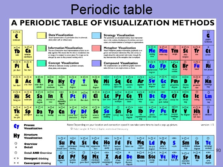
Periodic table 90

Managing visualization products • The importance of a ‘self-describing’ product • Visualization products are not just consumed by people • How many images, graphics files do you have on your computer for which the origin, purpose, use is still known? • How are these logically organized? 91

(Class 2) Management • • • Creation of logical collections Physical data handling Interoperability support Security support Data ownership Metadata collection, management and access. Persistence Knowledge and information discovery Data dissemination and publication 92

Use, citation, attribution • Think about and implement a way for others (including you) to easily use, cite, attribute any analysis or visualization you develop • This must include suitable connections to the underlying (aka backbone) data – and note this may not just be the full data set! • Naming, logical organization, etc. are key • Make them a resource, e. g. URI/ URL 93

Producability/ reproducability • The documentation around procedures used in the analysis and visualization are very often neglected – DO NOT make this mistake • Treat this just like a data collection (or generation) exercise • Follow your management plan • Despite the lack or minimal metadata/ metainformation standards, capture and record it • Get someone else to verify that it works 94

Summary • Purpose of analysis should drive the type that is conducted • Many constraints due to prior management of the data • Become proficient in a variety of methods, tools • Many considerations around visualization, similar to analysis, many new modes of viz. • Management of the products is a significant task 95

Reading • Note reading for week 7 – data sources for project definitions – There is a lot of material to review – Might be worth reviewing it before week 7 • Why – week 7 defines the group projects, come familiar with the data out there! Working with someone else's data 96

Reading assignment • Week 5 reading – is part retrospective and partly for week 8 – Worth reviewing - Data Analysis Tutorial • Note – for week 8 – Brief Introduction to Data Mining – Longer Introduction to Data Mining and slide sets – Software resources list – Example: Data Mining 97