Factor Analysis v PCA Peter Fox Data Analytics

Factor Analysis (v. PCA) Peter Fox Data Analytics – ITWS-4600/ITWS-6600 Week 10 a, April 5, 2016 1

Factor Analysis • Exploratory factor analysis (EFA) is a common technique in qualitative sciences for explaining the (shared) variance among several measured variables as a smaller set of latent (hidden/not observed) variables. • EFA is often used to consolidate survey data by revealing the groupings (factors) that underlie individual questions. • A large number of observable variables can be aggregated into a model to represent an underlying concept, making it easier to understand the data. 2

Examples • E. g. business confidence, morale, happiness and conservatism - variables which cannot be measured directly. • E. g. Quality of life. Variables from which to “infer” quality of life might include wealth, employment, environment, physical and mental health, education, recreation and leisure time, and social belonging. Others? • Tests, questionnaires, visual imagery… 3

Relation among factors • “correlated” (oblique) or “orthogonal” factors? • E. g. wealth, employment, environment, physical and mental health, education, recreation and leisure time, and social belonging • Relations? 4

Factor Analysis

PCA and FA? • CFA analyzes only the reliable common variance of data, while PCA analyzes all the variance of data. • An underlying hypothetical process or construct is involved in CFA but not in PCA. • PCA tends to increase factor loadings especially in a study with a small number of variables and/or low estimated communality. • Thus, PCA is not appropriate for examining the structure of data. 6

FA vs. PCA conceptually • FA produces factors; PCA produces components • Factors cause variables; components are aggregates of the variables

Conceptual FA and PCA

PCA and FA? • If the study purpose is to explain correlations among variables and to examine the structure of the data, FA provides a more accurate result. • If the purpose of a study is to summarize data with a smaller number of variables, PCA is the choice. • PCA can also be used as an initial step in FA because it provides information regarding the maximum number and nature of factors. – Scree plots (Friday) • More on this later… 9

The Relationship between Variables • Multiple Regression – Describes the relationship between several variables, expressing one variable as a function of several others, enabling us to predict this variable on the basis of the combination of the other variables • Factor Analysis – Also a tool used to investigate the relationship between several variables – Investigates whether the pattern of correlations between a number of variables can be explained by any underlying dimensions, known as ‘factors’ From: Laura Mc. Avinue School of Psychology Trinity College Dublin

Uses of Factor Analysis v. Test / questionnaire construction o o For example, you wish to design an anxiety questionnaire… Create 50 items, which you think measure anxiety Give your questionnaire to a large sample of people Calculate correlations between the 50 items & run a factor analysis on the correlation matrix o If all 50 items are indeed measuring anxiety… • All correlations will be high • One underlying factor, ‘anxiety’ v. Verification of test / questionnaire structure o Hospital Anxiety & Depression Scale o Expect two factors, ‘anxiety’ & ‘depression’

How does it work? • Correlation Matrix – Analyses the pattern of correlations between variables in the correlation matrix – Which variables tend to correlate highly together? – If variables are highly correlated, likely that they represent the same underlying dimension • Factor analysis pinpoints the clusters of high correlations between variables and for each cluster, it will assign a factor

Correlation Matrix Q 1 • • • Q 2 Q 3 Q 4 Q 5 Q 1 1 Q 2 . 987 1 Q 3 . 801 . 765 1 Q 4 -. 003 -. 088 0 1 Q 5 -. 051 . 044 . 213 . 968 1 Q 6 -. 190 -. 111 0. 102 . 789 . 864 Q 6 1 Q 1 -3 correlate strongly with each other and hardly at all with 4 -6 Q 4 -6 correlate strongly with each other and hardly at all with 1 -3 Two factors!

Factor Analysis • Two main things you want to know… – How many factors underlie the correlations between the variables? – What do these factors represent? • Which variables belong to which factors?

Steps of Factor Analysis 1. Suitability of the Dataset 2. Choosing the method of extraction 3. Choosing the number of factors to extract 4. Interpreting the factor solution

1. Suitability of Dataset v. Selection of Variables v. Sample Characteristics v. Statistical Considerations

Selection of Variables § Are the variables meaningful? • Factor analysis can be run on any dataset • ‘Garbage in, garbage out’ (Cooper, 2002) § Psychometrics • The field of measurement of psychological constructs • Good measurement is crucial in Psychology • Indicator approach • Measurement is often indirect • Can’t measure ‘depression’ directly, infer on the basis of an indicator, such as questionnaire § Based on some theoretical / conceptual framework, what are these variables measuring?

Selection of Variables, Example

How would you group these faces?

Sample Characteristics § Size § At least 100 participants § Participant : Variable Ratio § Estimates vary § Minimum of 5 : 1, ideal of 10 : 1 § Characteristics § Representative of the population of interest? § Contains different subgroups?

Statistical Considerations § Assumptions of factor analysis regarding data § Continuous § Normally distributed § Linear relationships § These properties affect the correlations between variables § Independence of variables § Variables should not be calculated from each other § e. g. Item 4 = Item 1 + 2 + 3

Statistical Considerations § Are there enough significant correlations (>. 3) between the variables to merit factor analysis? § Bartlett Test of Sphericity § Tests Ho that all correlations between variables = 0 § If p <. 05, reject Ho and conclude there are significant correlations between variables so factor analysis is possible

Statistical Considerations § Are there enough significant correlations (>. 3) between the variables to merit factor analysis? § Kaiser-Meyer-Olkin Measure of Sampling Adequacy § Quantifies the degree of inter-correlations among variables § Value from 0 – 1, 1 meaning that each variable is perfectly predicted by the others § Closer to 1 the better § If KMO >. 6, conclude there is a sufficient number of correlations in the matrix to merit factor analysis

Statistical Considerations, Example • All variables • • Continuous Normally Distributed Linear relationships Independent • Enough correlations? • Bartlett Test of Sphericity (χ2; df ; p <. 05) • KMO

2. Choosing the method of extraction v. Two methods v. Factor Analysis v. Principal Components Analysis v. Differ in how they analyse the variance in the correlation matrix

Variable Specific Error Variance unique to the variable itself Variance due to measurement error or some random, unknown source Common Variance that a variable shares with other variables in a matrix When searching for the factors underlying the relationships between a set of variables, we are interested in detecting and explaining the common variance

Principal Components Analysis • Ignores the distinction between the different sources of variance • Analyses total variance in the correlation matrix, assuming the components derived can explain all variance • Result: Any component extracted will include a certain amount of error & specific variance Factor Analysis V • Separates specific & error variance from common variance • Attempts to estimate common variance and identify the factors underlying this Which to choose? • Different opinions • Theoretically, factor analysis is more sophisticated but statistical calculations are more complicated, often leading to impossible results • Often, both techniques yield similar solutions

3. Choosing the number of factors to extract • Statistical Modelling – You can create many solutions using different numbers of factors • An important decision – Aim is to determine the smallest number of factors that adequately explain the variance in the matrix – Too few factors • Second-order factors – Too many factors • Factors that explain little variance & may be meaningless

Criteria for determining Extraction v. Theory / past experience v. Latent Root Criterion v. Scree Test v. Percentage of Variance Explained by the factors

Latent Root Criterion (Kaiser-Guttman) • Eigenvalues – Expression of the amount of variance in the matrix that is explained by the factor – Factors with eigenvalues > 1 are extracted – Limitations • Sensitive to the number of variables in the matrix • More variables… eigenvalues inflated… overestimation of number of underlying factors

Scree Test (Cattell, 1966) • Scree Plot – Based on the relative values of the eigenvalues – Plot the eigenvalues of the factors – Cut-off point • The last component before the slope of the line becomes flat (before the scree)

Elbow in the graph Take the components above the elbow

Percentage of Variance • Percentage of variance explained by the factors – Convention – Components should explain at least 60% of the variance in the matrix (Hair et al. , 1995)

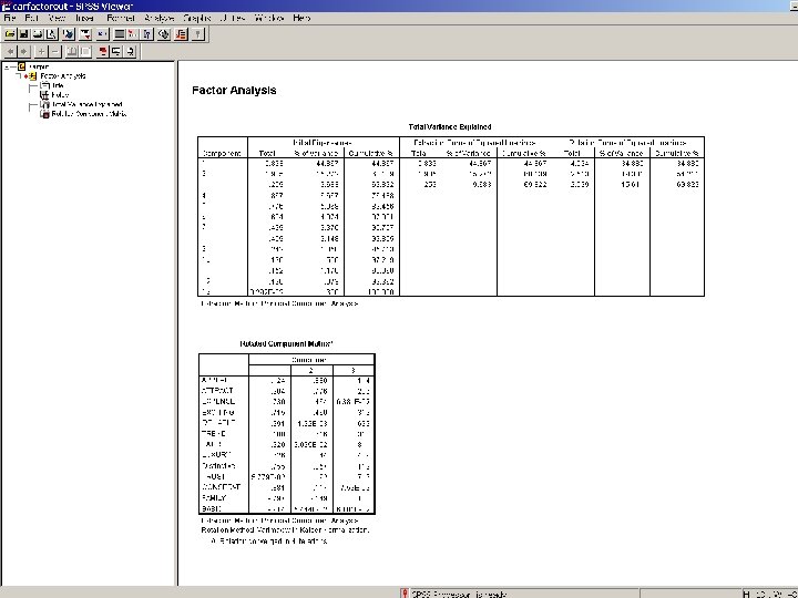
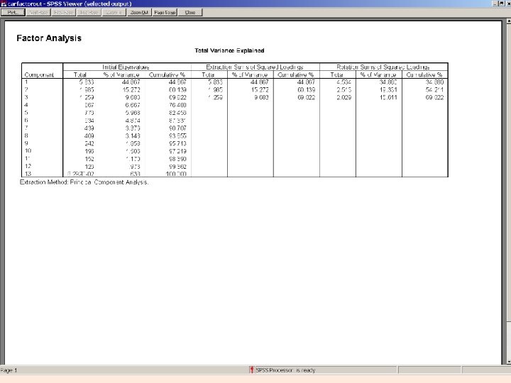
3. Choosing the number of factors to extract • Three components with eigenvalues > 1 • Explained 67. 26% of the variance

BFI data in psych (R) 35

4. Interpreting the Factor Solution • Factor Matrix – Shows the loadings of each of the variables on the factors that you extracted – Loadings are the correlations between the variables and the factors – Loadings allow you to interpret the factors • Sign indicates whether the variable has a positive or negative correlation with the factor • Size of loading indicates whether a variable makes a significant contribution to a factor – ≥. 3

Variables Component 1 Component 2 Component 3 Vividness Qu -. 198 -. 805 . 061 Control Qu . 173 . 751 . 306 Preference Qu . 353 . 577 -. 549 Generate Test -. 444 . 251 . 543 Inspect Test -. 773 . 051 -. 051 Maintain . 734 -. 003 . 384 Transform(P&P) Test . 759 -. 155 . 188 Transform (Comp) Test -. 792 . 179 . 304 Visual STM Test . 792 -. 102 . 215 Component 1 – Visual imagery tests Component 2 – Visual imagery questionnaires Component 3 – ?

Factor Matrix • Interpret the factors • Communality of the variables – Percentage of variance in each variable that can be explained by the factors • Eigenvalues of the factors – Helps us work out the percentage of variance in the correlation matrix that the factor explains

Component 1 Component 2 Component 3 Communality Vividness Qu -. 198 -. 805 . 061 69% Control Qu . 173 . 751 . 306 69% Preference Qu . 353 . 577 -. 549 76% Generate Test -. 444 . 251 . 543 55% Inspect Test -. 773 . 051 -. 051 60% Maintain . 734 -. 003 . 384 69% Transform (P&P) Test . 759 -. 155 . 188 64% Transform (Comp) Test -. 792 . 179 . 304 75% Visual STM Test . 792 -. 102 . 215 69% Eigenvalues 3. 36 1. 677 1. 018 / % Variance 37. 3% 18. 6% 11. 3% / Variables Communality of Variable 1 (Vividness Qu) = (-. 198)2 + (-. 805)2 + (. 061)2 =. 69 or 69% Eigenvalue of Comp 1 = ( [-. 198]2 + [. 173]2 + [. 353]2 + [-. 444]2 + [. 773]2 +[. 734]2 + [. 759]2 + [-. 792]2 + [. 792]2 ) = 3. 36 / 9 = 37. 3%

Factor Matrix • Unrotated Solution – Initial solution – Can be difficult to interpret – Factor axes are arbitrarily aligned with the variables • Rotated Solution – Easier to interpret – Simple structure – Maximises the number of high and low loadings on each factor

Factor Analysis through Geometry • It is possible to represent correlation matrices geometrically • Variables – Represented by straight lines of equal length – All start from the same point – High correlation between variables, lines positioned close together – Low correlation between variables, lines positioned further apart – Correlation = Cosine of the angle between the lines

V 1 & V 3 V 1 90º angle V 2 Cosine = 0 No relationship 30º 60º V 3 The smaller the angle, the bigger the cosine and the bigger the correlation V 1 & V 2 30º angle Cosine =. 867 r =. 867 V 2 & V 3 60º angle Cosine =. 5 R =. 5

F 1 V 2 V 3 Factor Analysis Fits a factor to each cluster of variables V 4 V 5 V 6 F 2 Factor Loading Cosine of the angle between each factor and the variable Passes a factor line through the groups of variables

Two Methods of fitting Factors F 1 V 1 V 2 V 3 V 4 V 5 V 6 F 2 Orthogonal Solution Oblique Solution Factors are at right angles Factors are not at right angles Uncorrelated Correlated F 2

Two Step Process F 1 V 1 V 2 V 1 V 3 V 4 V 5 V 6 Factors are fit arbitrarily V 2 V 3 F 2 V 5 F 2 V 6 Factors are rotated to fit the clusters of variables better

For example… Solution following Orthogonal Rotation Unrotated Solution Variables C 1 C 2 C 3 Vividness Qu -. 198 -. 805 . 061 Vividness Qu -. 029 -. 831 . 008 Control Qu . 173 . 751 . 306 Control Qu . 174 . 744 . 323 Preference Qu . 353 . 577 -. 549 Preference Qu -. 010 . 679 -. 547 Generate Test -. 444 . 251 . 543 Generate Test -. 197 . 112 . 709 Inspect Test -. 773 . 051 -. 051 Inspect Test -. 717 -. 103 . 279 Maintain Test . 734 -. 003 . 384 Maintain Test . 819 . 116 . 043 Transform (P&P) Test . 759 -. 155 . 188 Transform (P&P) Test . 779 -. 013 -. 166 Transform (Comp) Test -. 792 . 179 . 304 Transform (Comp) Test -. 599 -. 01 . 626 Visual STM Test . 792 -. 102 . 215 Visual. STM Test . 813 . 045 -. 147

Factor Rotation • Changes the position of the factors so that the solution is easier to interpret • Achieves simple structure – Factor matrix where variables have either high or low loadings on factors rather than lots of moderate loadings

Evaluating your Factor Solution • Is the solution interpretable? – Should you re-run and extract a bigger or smaller number of factors? • What percentage of variance is explained by the factors? – >60%? • Are all variables represented by the factors? – If the communality of one variable is very low, suggests it is not related to the other variables, should re-run and exclude

For example… First Solution Variables Vividness Qu Control Qu Preference Qu C 1 -. 029. 174 -. 010 C 2 -. 831. 744. 679 Second Solution C 3 Component 1 Component 2 Vividness Qu . 013 -. 829 Control Qu -. 023 . 770 Preference Qu . 195 . 648 Generate Test -. 493 . 130 Inspect Test -. 760 -. 146 Maintain Test . 711 . 183 Transform (P&P) Test . 773 . 042 Transform Test -. 811 -. 028 . 792 . 103 . 008. 323 -. 547 Generate Test -. 197 . 112 . 709 Inspect Test -. 717 -. 103 . 279 Maintain Test . 819 . 116 . 043 Transform (P&P) Test . 779 -. 013 -. 166 Transform (Comp) Test -. 599 -. 01 . 626 Visual. STM Test . 813 . 045 -. 147 Component 3 = ? Variables (Comp) Visual STM Test C 1 = Efficiency of objective visual imagery C 2 = Self-reported imagery efficacy

Cumulative percent of variance explained. We are looking for an eigenvalue above 1. 0.

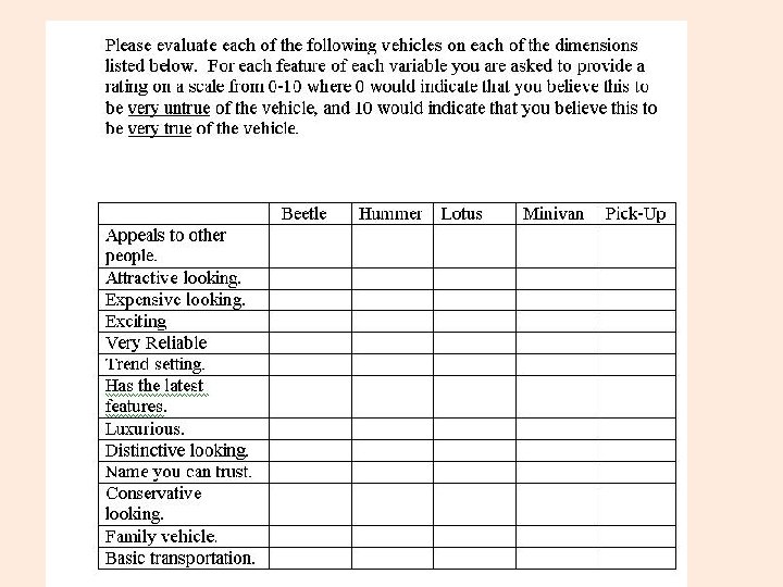
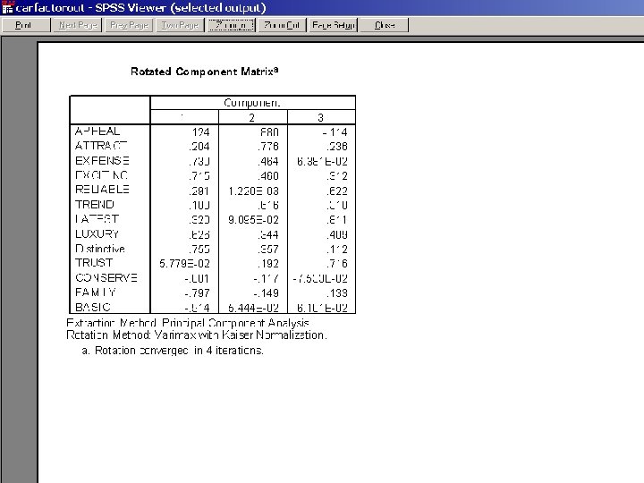
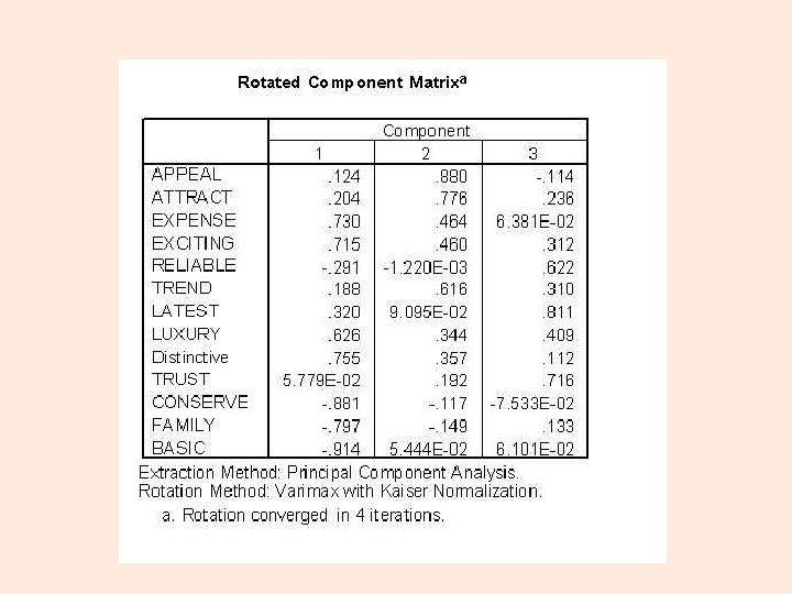
Expensive Appeals to Others Reliable Exciting Attractive Looking Latest Features Luxury Trend Setting Trust Distinctive Not Conservative Not Family Not Basic

What shall these components be called? Expensive Appeals to Others Reliable Exciting Attractive Looking Latest Features Luxury Trend Setting Trust Distinctive Not Conservative Not Family Not Basic

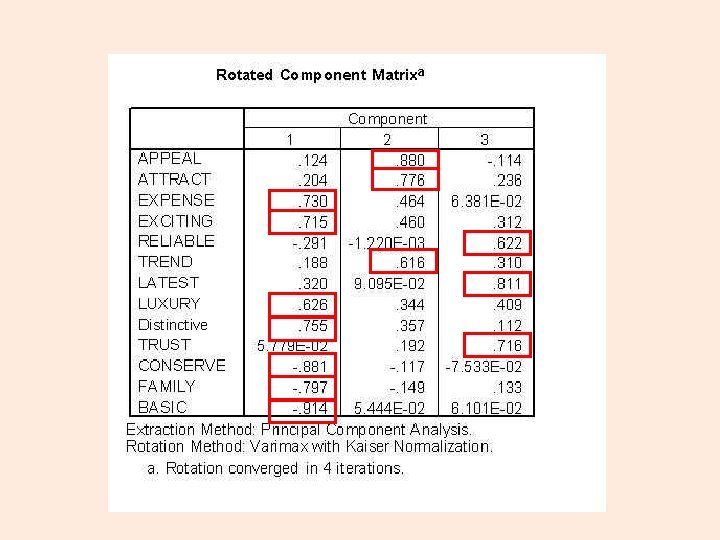
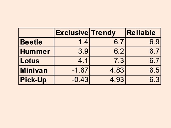
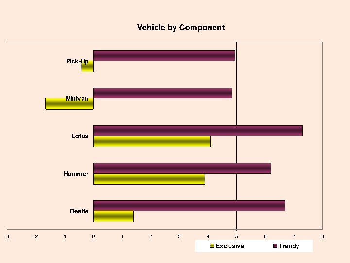
EXCLUSIVE TRENDY RELIABLE Expensive Appeals to Others Reliable Exciting Attractive Looking Latest Features Luxury Trend Setting Trust Distinctive Not Conservative Not Family Not Basic

Calculate Component Scores EXCLUSIVE = (Expensive + Exciting + Luxury + Distinctive – Conservative – Family – Basic)/7 TRENDY = (Appeals to Others + Attractive Looking + Trend Setting)/3 RELIABLE = (Reliable + Latest Features + Trust)/3

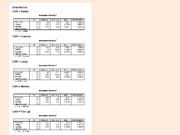
Not much differing on this dimension.

References • Some… • Cooper, C. (1998). Individual differences. London: Arnold. • Kline, P. (1994). An easy guide to factor analysis. London: Routledge.

Assignments • Assignment 7: Predictive and Prescriptive Analytics. Due ~ week ~12. 20%. . 67