CSC 41513 Intro to Algorithms LinearTime Sorting Algorithms

CSC 41/513: Intro to Algorithms Linear-Time Sorting Algorithms

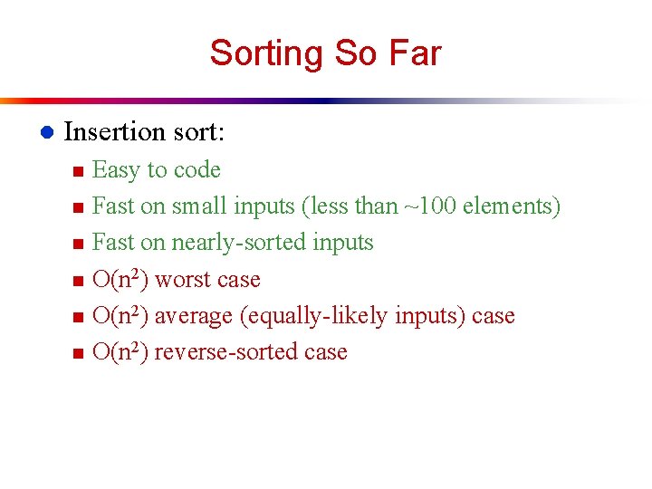
Sorting So Far l Insertion sort: n n n Easy to code Fast on small inputs (less than ~100 elements) Fast on nearly-sorted inputs O(n 2) worst case O(n 2) average (equally-likely inputs) case O(n 2) reverse-sorted case

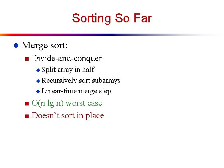
Sorting So Far l Merge sort: n Divide-and-conquer: u Split array in half u Recursively sort subarrays u Linear-time merge step n n O(n lg n) worst case Doesn’t sort in place

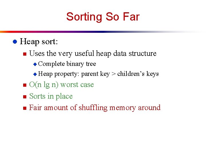
Sorting So Far l Heap sort: n Uses the very useful heap data structure u Complete binary tree u Heap property: parent key > children’s keys n n n O(n lg n) worst case Sorts in place Fair amount of shuffling memory around

Sorting So Far l Quick sort: n Divide-and-conquer: u Partition array into two subarrays, recursively sort u All of first subarray < all of second subarray u No merge step needed! n n n O(n lg n) average case Fast in practice O(n 2) worst case u Naïve implementation: worst case on sorted input u Address this with randomized quicksort

How Fast Can We Sort? We will provide a lower bound, then beat it l First, an observation: all of the sorting algorithms so far are comparison sorts l n n The only operation used to gain ordering information about a sequence is the pairwise comparison of two elements Theorem: all comparison sorts are (n lg n) u. A comparison sort must do O(n) comparisons (why? ) u What about the gap between O(n) and O(n lg n)

Decision Trees l Decision trees provide an abstraction of comparison sorts n A decision tree represents the comparisons made by a comparison sort. Every thing else ignored What do the leaves represent? l How many leaves must there be? l

Decision Trees l Decision trees can model comparison sorts. For a given algorithm: n n n One tree for each n Tree paths are all possible execution traces What’s the longest path in a decision tree for insertion sort? For merge sort? What is the asymptotic height of any decision tree for sorting n elements? l Answer: (n lg n) (now let’s prove it…) l

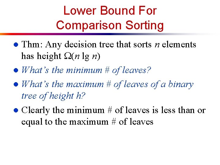
Lower Bound For Comparison Sorting Thm: Any decision tree that sorts n elements has height (n lg n) l What’s the minimum # of leaves? l What’s the maximum # of leaves of a binary tree of height h? l Clearly the minimum # of leaves is less than or equal to the maximum # of leaves l

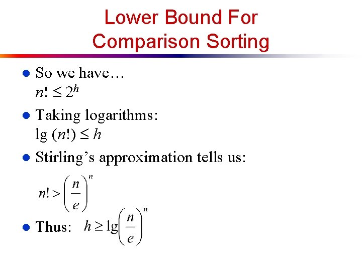
Lower Bound For Comparison Sorting So we have… n! 2 h l Taking logarithms: lg (n!) h l Stirling’s approximation tells us: l l Thus:

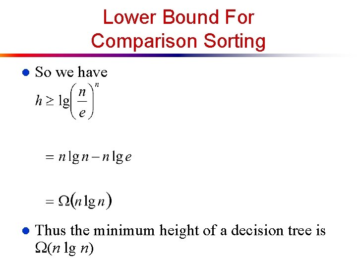
Lower Bound For Comparison Sorting l So we have l Thus the minimum height of a decision tree is (n lg n)

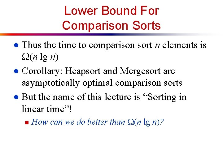
Lower Bound For Comparison Sorts Thus the time to comparison sort n elements is (n lg n) l Corollary: Heapsort and Mergesort are asymptotically optimal comparison sorts l But the name of this lecture is “Sorting in linear time”! l n How can we do better than (n lg n)?

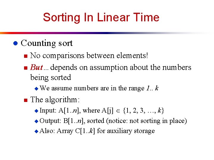
Sorting In Linear Time l Counting sort n n No comparisons between elements! But…depends on assumption about the numbers being sorted u We n assume numbers are in the range 1. . k The algorithm: A[1. . n], where A[j] {1, 2, 3, …, k} u Output: B[1. . n], sorted (notice: not sorting in place) u Also: Array C[1. . k] for auxiliary storage u Input:

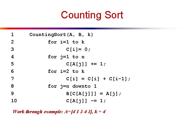
Counting Sort 1 2 3 4 5 6 7 8 9 10 Counting. Sort(A, B, k) for i=1 to k C[i]= 0; for j=1 to n C[A[j]] += 1; for i=2 to k C[i] = C[i] + C[i-1]; for j=n downto 1 B[C[A[j]]] = A[j]; C[A[j]] -= 1; Work through example: A={4 1 3 4 3}, k = 4

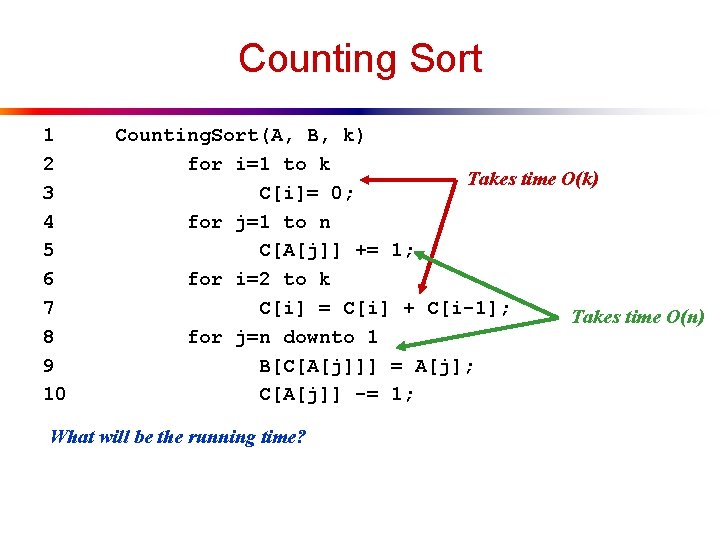
Counting Sort 1 2 3 4 5 6 7 8 9 10 Counting. Sort(A, B, k) for i=1 to k Takes time O(k) C[i]= 0; for j=1 to n C[A[j]] += 1; for i=2 to k C[i] = C[i] + C[i-1]; Takes time O(n) for j=n downto 1 B[C[A[j]]] = A[j]; C[A[j]] -= 1; What will be the running time?

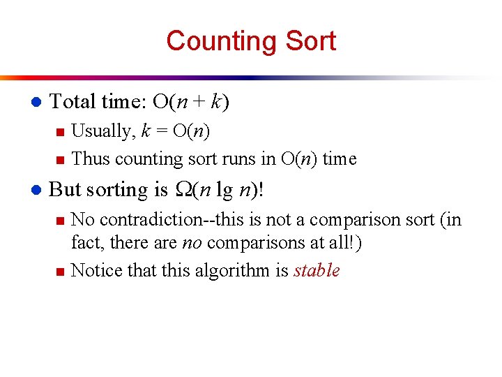
Counting Sort l Total time: O(n + k) n n l Usually, k = O(n) Thus counting sort runs in O(n) time But sorting is (n lg n)! n n No contradiction--this is not a comparison sort (in fact, there are no comparisons at all!) Notice that this algorithm is stable

Counting Sort Why don’t we always use counting sort? l Because it depends on range k of elements l Could we use counting sort to sort 32 bit integers? Why or why not? l Answer: no, k too large (232 = 4, 294, 967, 296) l

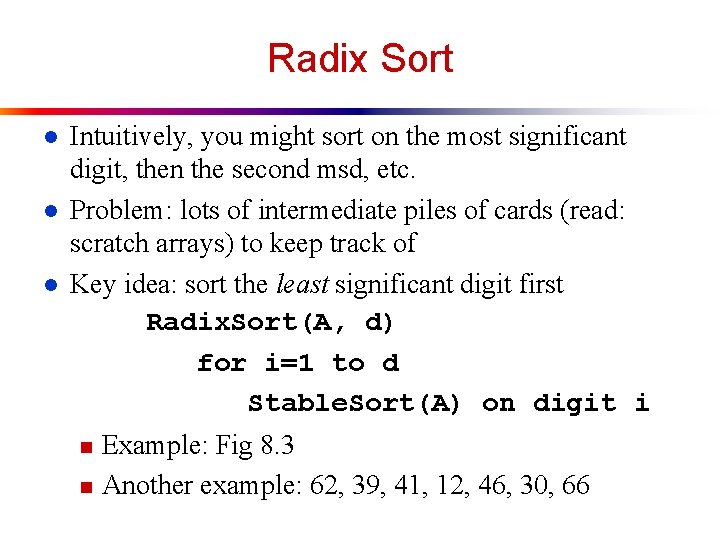
Radix Sort l l l Intuitively, you might sort on the most significant digit, then the second msd, etc. Problem: lots of intermediate piles of cards (read: scratch arrays) to keep track of Key idea: sort the least significant digit first Radix. Sort(A, d) for i=1 to d Stable. Sort(A) on digit i n n Example: Fig 8. 3 Another example: 62, 39, 41, 12, 46, 30, 66

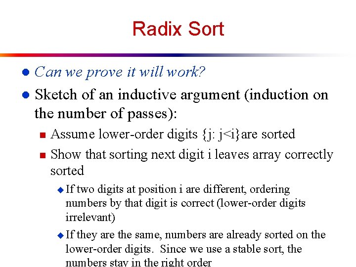
Radix Sort Can we prove it will work? l Sketch of an inductive argument (induction on the number of passes): l n n Assume lower-order digits {j: j<i}are sorted Show that sorting next digit i leaves array correctly sorted u If two digits at position i are different, ordering numbers by that digit is correct (lower-order digits irrelevant) u If they are the same, numbers are already sorted on the lower-order digits. Since we use a stable sort, the numbers stay in the right order

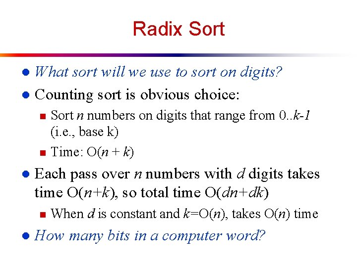
Radix Sort What sort will we use to sort on digits? l Counting sort is obvious choice: l n n l Each pass over n numbers with d digits takes time O(n+k), so total time O(dn+dk) n l Sort n numbers on digits that range from 0. . k-1 (i. e. , base k) Time: O(n + k) When d is constant and k=O(n), takes O(n) time How many bits in a computer word?

Radix Sort l Problem: sort 1 million 64 -bit numbers n n l Compares well with typical O(n lg n) comparison sort n l Treat as four-digit radix 216 numbers Can sort in just four passes with radix sort! Requires approx lg n = 20 operations per number being sorted So why would we ever use anything but radix sort?

Radix Sort l In general, radix sort based on counting sort is n n l Fast Asymptotically fast (i. e. , O(n)) Simple to code A good choice To think about: Can radix sort be used on floating-point numbers?

Bucket Sort l Bucket sort n n Assumption: input is n reals from [0, 1) Basic idea: u Create n linked lists (buckets) to divide interval [0, 1) into subintervals of size 1/n u Add each input element to appropriate bucket and sort buckets with insertion sort n Uniform input distribution O(1) bucket size u Therefore n the expected total time is O(n) These ideas will return when we study hash tables

The End