CS565 Computer Vision Nazar Khan Lecture 2 A

CS-565 Computer Vision Nazar Khan Lecture 2

A Note on Pre-Requisites • Some students are concerned about the pre-requisites – Linear Algebra – Probability – Calculus • We will cover some basics as they come along. • So don’t worry too much. • However, it will serve you well to read the Appendices of standard Computer Vision, Image Processing or Computer Graphics books. They are usually very helpful – Appendix from Rich Szeliski’s book – Appendix from Gonzalez & Woods’ book

Topics to be covered • Image types • Sampling and Quantization • Noise models

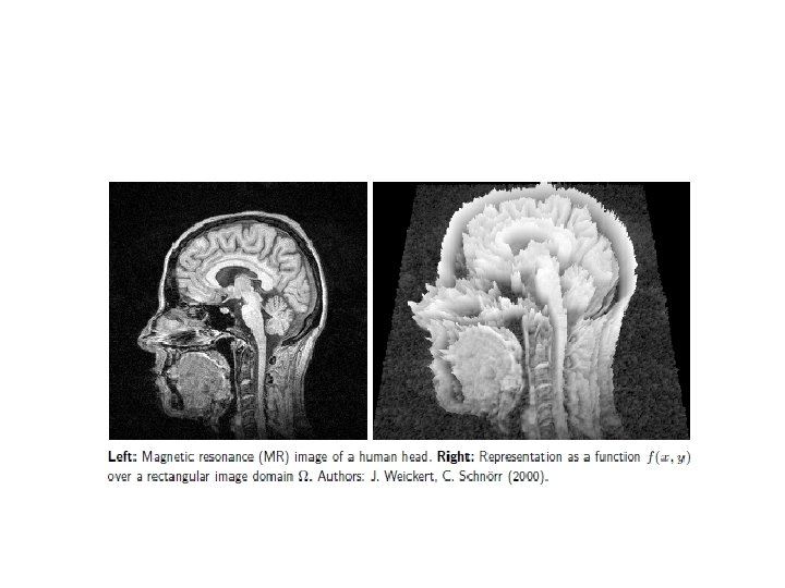
Image Concepts • What is a grayscale image? – A mapping from a rectangular domain to the range • The domain is called image domain or image plane • The range specifies grey value • Usually low grey values are dark and high grey values bright.

Sampling • • Discretization of the domain Image data lie on a rectangular grid of points This creates a digital image Grid point is called a pixel (picture element) – Pixel dimensions are usually the same in both directions. • Sampling determines image quality

Sampling

Quantization • Discretization of the range • Saves disk space • If gray value is coded by a single byte, then the discrete range is given by? – {0, 1, …, 255} • Range of binary images? – {0, 1} • Humans can distinguish only 40 grayscales • But we are also very good at analyzing binary images.

Quantization

Image Types • • • m-dimensional images Domain in m=1: signals m=2: 2 D images m=3: 3 D images (CT Scan, MRI, Kinect) – Image points in 3 D are called voxels (volume elements) – Voxel dimensions usually differ in different directions.

Image Types

Image Types • • Vector Valued Images Range in Equivalent to having channels Examples: – Color Images • 3 channels – Red, Green Blue • Humans can distinguish 2, 000 colours! – Multispectral images • Satellite images • Many channels (4 -30) that represent different frequency bands.

Image Types • Matrix valued images • Range in • Every pixel location stores an n-by-n matrix – Useful in medical imaging

Image Types • Image Sequences • Any of the above types of images can be considered in sequence • Domain will change from Rm to Rm+1. • For this class, we will mainly be concerned with 2 D grayscale images and/or this sequences.

NOISE MODELS

Noise Models • Noise – Additive Noise – Multiplicative Noise – Impulse Noise – Measuring Noise • Blur – Convolutions – Modelling Blur by Convolutions • Combined Blur and Noise

Noise • Very common in digital images (or any realworld data) • Can have many reasons, e. g. – image sensor of a digital camera – grainy photographic films that are digitised – specific acquisition methods: • e. g. ultrasound imaging always creates ellipse-shaped speckle noise – atmospheric disturbance during wireless transmission

Additive Noise • Most important type of noise – F=G+N where G is the original image and N is the noise. • Distribution of N – Uniform (pretty easy) – Gaussian (pretty common)

Uniform Additive Noise • • Not a very realistic model of noise But easy to simulate Constant density function between a and b F=G+U where every pixel in U is uniformly distributed between a and b

Uniform Additive Noise

Gaussian Additive Noise • Most important noise model – thermal noise from the image sensor – circuit noise from signal amplifications • When many sources of noise are combined, the cumulative noise can be modeled using a Gaussian density • F=G+

Gaussian Additive Noise • Gaussian noise lies almost completely within the interval

Gaussian Additive Noise

Multiplicative Noise • Signal dependent – noise caused by grains of a photographic emulsion • F=G+N. *G

Multiplicative Noise

Impulse Noise • Degrades only some pixels. – Additive and multiplicative noise affects all pixels – Defect in the imaging sensor • Unipolar – defective pixels have the same wrong gray value • Bipolar – defective pixels can have either of 2 wrong gray values – salt-and-pepper noise – max and min gray value

Impulse Noise

Measuring Noise • Mean Squared Error: – The smaller the better • Peak-Signal-to-Noise Ratio: – The higher the better – Unit is decibel (d. B) – PSNR <30 d. B starts to become noticeable

Measuring Noise

Blur • Second source of image degradation besides noise – Defocusing, imperfections of the optical system, motion blur • Simplest blur – shift invariant (same amount of blurring at all image locations) • Can be thought of as a weighted averaging within a certain neighbourhood

Blur • Weighted Averaging Convolution

Convolution

Convolution • Properties