CS 565 Computer Vision Nazar Khan Lecture 11

CS 565 Computer Vision Nazar Khan Lecture 11

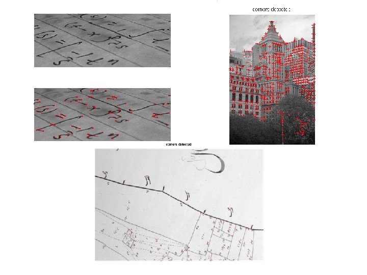
What is a Corner? • A corner may be interpreted as an intersection of two edges, or as a region where strong derivatives exist in more than one direction

Corner Detection • The gradient vector is sufficient to give the local structure information for an edge. • For corners, the local structure direction around the corner changes strongly. – This suggests that corner phenomenon requires looking in a neighbourhood. • We want to find the directions of largest/smallest grayvalue changes within a neighbourhood. • This requires integration of directional information over a neighbourhood.

Corner Detection • Let ∇u be the gradient direction. • A vector n that is orthogonal to ∇u satisfies n. T∇u=0. • Let us average the gradient ∇u. N vectors in a certain neighbourhood N. – ∑N ∇u • A vector n that is “most orthogonal” to the average gradient direction within a neighbourhood N • Is a minimiser of E(n)=∑N (n. T∇u)2

Corner Detection E(n) = = where A ∑N (n. T∇u)2 ∑N n. T∇u∇u. Tn n. T (∑N ∇u∇u. T ) n n. T An = ∑N ∇u∇u. T = [ux 2 uxuy ; uxuy uy 2].

Some Linear Algebra • Let n be a unit vector. • n. T An is projection of n onto An • This projection will be maximum when An has the same direction as n. • Vectors n for which An has the same direction are known as eigen-vectors of A. – An=λn where λ is the eigen-value corresponding to the eigen-vector n. – For the largest eigen-value of A, n. T An = λ 1. – For the smallest eigen-value of A, n. T An = λ 2.

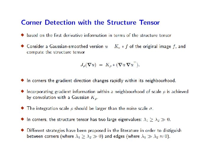
Structure Tensor The matrix of summations A = ∑N ∇u∇u. T = [ ∑N u x 2 ∑N u x u y ] [ ∑N u x u y ∑N u y 2 ] is often replaced by the matrix of Gaussian averages Jρ = Kρ * (∇u∇u. T) [ Kρ*ux 2 Kρ*(uxuy) ] [ Kρ*(uxuy) Kρ*uy 2 ] which is the so-called structure tensor. Captures changes in local structure around a point.

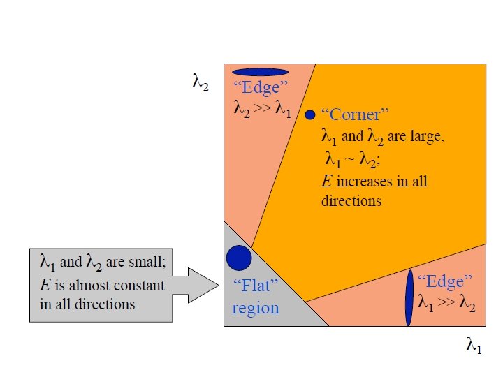
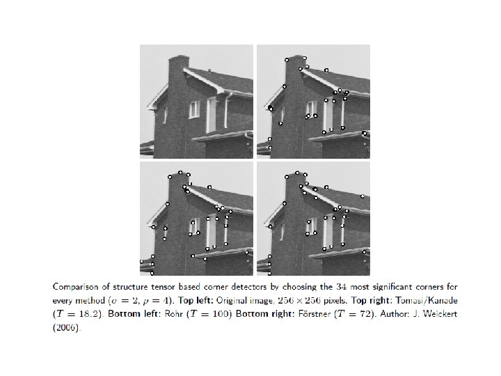
Structure Tensor • The structure tensor Jρ is – Symmetric – Positive definite • Its orthonormal eigenvectors v 1, v 2 specify the directions of largest/smallest contrast within some integration scale ρ. • The corresponding eigenvalues λ 1, λ 2 describe the average contrast along these directions. • Let λ 1>= λ 2. The eigenvalues allow a useful analysis of the local image structure: – – constant areas: λ 1 = λ 2 = 0 straight edges: λ 1 >> λ 2 = 0 corners: λ 1 >= λ 2 >> 0 measure of anisotropy: (λ 1 - λ 2)2

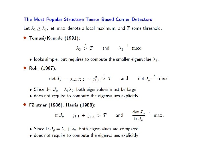
Harris Corner Detector • Approximation 24

25

26

27

28

29

Corner Detection – A Second Look • A corner is different from its surroundings. • A patch placed on a corner pixel is different from its surrounding patches. Patch is similar to patches in all directions Patch is similar to patches in vertical direction Patch is similar to patches in horizontal direction Patch is NOT similar to patches in all directions

+ + - Demo of a point + with well distinguished neighbourhood. >0

+ + - Demo of a point + with well distinguished neighbourhood. >0

+ + - Demo of a point + with well distinguished neighbourhood. >0

+ + - Demo of a point + with well distinguished neighbourhood. >0

+ + - Demo of a point + with well distinguished neighbourhood. >0

+ + - Demo of a point + with well distinguished neighbourhood. >0

+ + - Demo of a point + with well distinguished neighbourhood. >0

+ + - Demo of a point + with well distinguished neighbourhood. >0

Patch Similarity • Similarity of two patches p and q can be computed via the sum-of-squared-differences (SSD). • SSD(p, q)=∑(pij-qij)2

Moravec Corner Detector • Among the early corner detection approaches. • Basic Idea: A corner should have low selfsimilarity. – Self-similarity: how similar a patch is to neighbouring, overlapping patches. • Corner Strength: min(SSD(p, q. N )) – If p is different from its neighbours in all directions, then this min value will be large. • If corner strength at a pixel is locally maximal, then this pixel is a corner.

Moravec Corner Detector • Weakness: If an edge is not aligned with the directions we are looking in, then this edge will be falsely detected as a corner. Directions that we look in Patch is NOT similar to patches in all directions that we look in. So it will be detected as a corner instead of an edge pixel.

Harris Corner Detector • Solution: – Do not fix the directions that we are looking in. – Find the direction in which patches become most dissimilar. • That is, the direction that maximises the SSD from current patch.

Harris Corner Detector d* H. W. : Prove that these two expressions are equivalent.

Harris Corner Detector d*

Harris Corner Detector d*

Harris Corner Detector • What is the difference between d* and gradient direction u? – Gradient u is for a pixel. – d* is for a patch. d*

Harris Corner Detector • For an edge, the direction orthogonal to d* will be the direction of least change in our weighted SSD. – From S(d)=d. TAd= , the weighted SSD in direction d* is given by the corresponding eigenvalue. • Since the structure tensor A is symmetric, positive definite, its eigenvectors will be orthonormal. • So the direction of least change in weighted SSD is given by the 2 nd eigenvector of A. – the weighted SSD in this direction is given by the corresponding eigenvalue. • If this eigenvalue is large, then we have a nonedge/corner.

Harris Corner Detector • If the smaller eigenvalue is large, then we have a non-edge/corner. • large small 0 flat region • large>> small 0 edge • large and small >> 0 corner

Harris Corner Detector Author: Nazar Khan (2014)

Harris Corner Detector V 1 V 2 Corner Author: Nazar Khan (2014)

Harris Corner Detector V 1 V 2 Corner Author: Nazar Khan (2014)

Corner Detection • H. W: Write a detailed derivation/explanation of the Harris corner detector starting from the Moravec corner detector. • H. W: Implement a simple Harris corner detector using the rule small>T and test it on some sample real-world image. – Experiment with other corner measures: • Haris & Stpehens • Shi-Tomasi • Nobel