CS 565 Computer Vision Nazar Khan Lecture 9

CS 565 Computer Vision Nazar Khan Lecture 9

Linear Shift-Invariant Filtering • We have studied convolution in Lecture 4. • Convolution is 1. Linear: (�f+ βg)*w = �f*w+ βg*w for �, β in R. • 2. Convolution of linear combination equals linear combination of convolutions. Shift-invariant: Tb(f*w) = Tbf*w for translation Tb in R. • 3. Translating the signal is equivalent to translating the convolution. Commutative: f*w = w*f • 4. Signal and filter play an equal role. Associative: (f*v)*w = f*(v*w) • Successive convolutions with kernels v and w equal a single convolution by the kernel v*w. • Any filter obeying properties 1 and 2 is called a Linear Shift-Invariant (LSI) filter.

Derivative Filtering • Derivative filters are an important special case of LSI filters. • Derivatives capture local gray value image changes. – Perceptually important features such as edges and corners. • Derivative computation can be dangerous.

Derivative Filtering Left: A road image for which two 1 D signals along the red and blue horizontal scan-lines have been extracted. Right: The intensity profiles along the red and blue scan-lines. The large jumps in the profiles correspond to boundaries of trees and road. Author: Nazar Khan (2014)

Derivative Filtering 1 D signal 1 st Derivative 2 nd Derivative Edge corresponds to maximum of 1 st derivative magnitude. Edge corresponds to zero-crossing of 2 nd derivative.

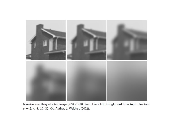
Derivative computation can be dangerous • Noise can be amplified. – This leads to false edges. • Derivatives in spatial domain become multiplications with frequency in Fourier domain. – High frequency (noise) components get amplified. H. W. : Prove this. • Solution: remove high frequencies before computing derivatives (often done through Gaussian convolution).

Left: A 1 D intensity profile. Right: Plot of the 2 nd derivatives. The small preturbations (noise) in the input lead to false zero-crossings (edges) in 2 nd derivatives. Author: Nazar Khan (2014)

Average vs Derivative Filtering • Average – All values are +ve – Sum to 1 – Output on smooth region is unchanged – Blurs areas of high contrast – Larger mask -> more smoothing • Derivative – opposite signs – Sum to zero – Output on smooth region is zero – Gives high output in areas of high contrast – Larger mask -> more edges detected

Some Notation From 2 D Calculus • Let f(x, y) be a 2 D function. • ∂f/∂x = ∂xf = fx is the partial derivative of f with respect to x while keeping y fixed. – ∂2 f/∂x∂y = ∂/∂x (∂f/∂y) – fxy=fyx (under suitable smoothness assumptions).

Some Notation From 2 D Calculus • Nabla operator ∇ or gradient is the column vector of partial derivatives ∇=(∂x, ∂y). • ∇f=(∂xf, ∂yf ) points in the direction of steepest ascent. • |∇f|=sqrt(fx 2+fy 2) is invariant under rotations. • Laplacian operator ∆f = fxx+fyy – Sum of 2 nd derivatives

Discrete Derivative Approximations • Let h be the grid distance. For grids of image pixels, usually h=1. fi-1 fi fi+1 • 1 st derivative approximation – Forward difference fi’=(fi+1 -fi )/h – Backward difference fi’=(fi-fi-1 )/h – Central difference fi’= (fi+1 -fi-1)/2 h • 2 nd derivative approximation – Central difference fi’= (fi+1 -2 fi+fi-1)/2 h

Discrete Derivative Approximations • Taking central differences is better. • In 2 D, use ∂2 f/∂x∂y = ∂/∂x (∂f/∂y). • Convolve in one direction, then convolve the result in the other. This way, we carry out 2 D convolutions using 1 D convolutions only.

Discrete 2 D Laplacian Approximation • A standard approximation of the 2 D Laplacian ∆f = fxx+fyy is given by • The true Laplacian is rotationally invariant but this discrete approximation is not.

Discrete 2 D Laplacian Approximation • A better, rotationally invariant discrete approximation of the Laplacian is given by

Edge Detection • Edge – strong change in local neighbourhood. • One of the most important image features. • We can understand comics and line drawings. • Edge detection is the first step from low-level vision (pixel based descriptors) towards high-level vision (image content). • Can be detected through 1 st or 2 nd order derivative operators.

Edge Detection via 1 st Order Derivatives 1. Reduce high frequencies (noise) in image f by convolving with a Gaussian kernel Kσ. Smooth image u= Kσ*f. 2. Compute approximate 1 st derivatives ux and uy and compute gradient magnitude |∇u|=sqrt(ux 2+uy 2) 3. Edge pixels correspond to |∇u|>T.

Clockwise from top-left: Original image I, horizontal derivative image Ix, vertical derivative image Iy, gradient magnitude image |∇u|, |∇u|>5, |∇u|>10. Author: Nazar Khan (2014)

Edge Detection via 1 st Order Derivatives • Advantage – 1 st order derivatives are more robust to noise than 2 nd order derivatives. • Disadvantages – Require threshold parameter T. Some edges may be below T. – Some edges may be too thick. • Remarks – Suitable T strongly depends on σ. Why? – T can be selected as a suitable percentile of the histogram of |∇u|. • T is the 75 th percentile if |∇u|<T for 75% of the pixels.

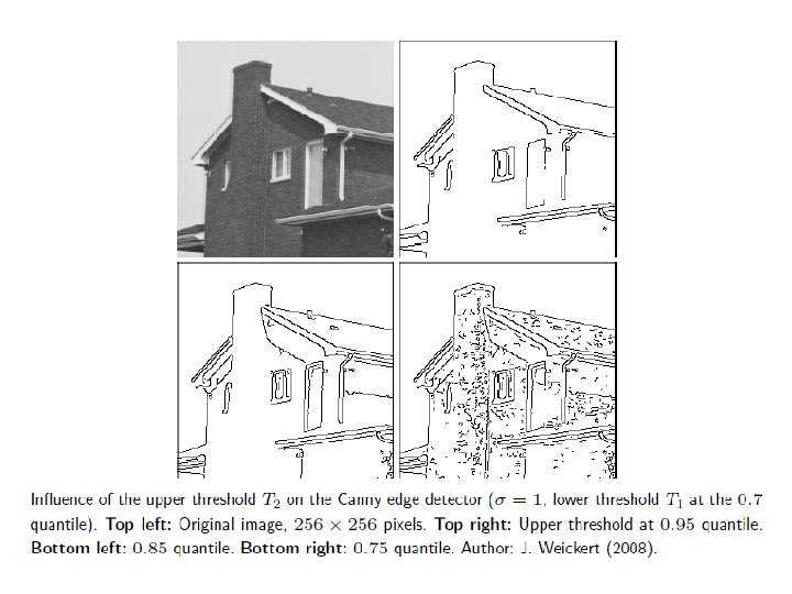
Canny Edge Detector • • Among the best performing edge detectors. Mainly due to sophisticated post-processing. 3 main steps. 3 parameters – Standard deviation σ of Gaussian smoothing kernel. – Two thresholds Tlow and Thigh.

Canny Edge Detector 1. Gradient approximation by Gaussian derivatives – Magnitude |∇u|=sqrt(ux 2+uy 2) – Orientation angle φ=arg(|∇u|)=atan(ux, uy) – |∇u|>Tlow are candidate edge pixels. 2. Non-maxima Suppression (thinning of edges to a width of 1 pixel) – In every edge candidate, consider the grid direction (out of 4 directions) that is “most orthogonal” to the edge. – Basic Idea: If one of the two neighbours in this direction has a larger gradient magnitude, mark the central pixel. – After passing through all candidates, remove marked pixels from the edge map.

Non-maxima Suppression • Quantisation of gradient direction.

Non-maxima Suppression Only this point remains. The remaining magnitudes along the line are set to 0. Remove all points along the gradient direction that are not maximum points.

Original Quantized φ Gradient magnitude |∇u| Gradient direction φ Non-maxima suppression of |∇u|

Canny Edge Detector 3. Hysteresis Thresholding (Double Thresholding): – Basic Idea: If a weak edge lies adjacent to a strong edge, include the weak edge too. – Use pixels above upper threshold Thigh as seed points for relevant edges. – Recursively add all neighbours of seed points that are above the lower threshold Tlow.

Hysteresis Thresholding • Scan image from left to right, top to bottom • If M(x, y) is above Thigh mark it as edge. • Recursively look at neighbors; if gradient magnitude is above Tlow mark it as edge.

Gradient Magnitude Hysteresis Thresholding High Low Neighbours

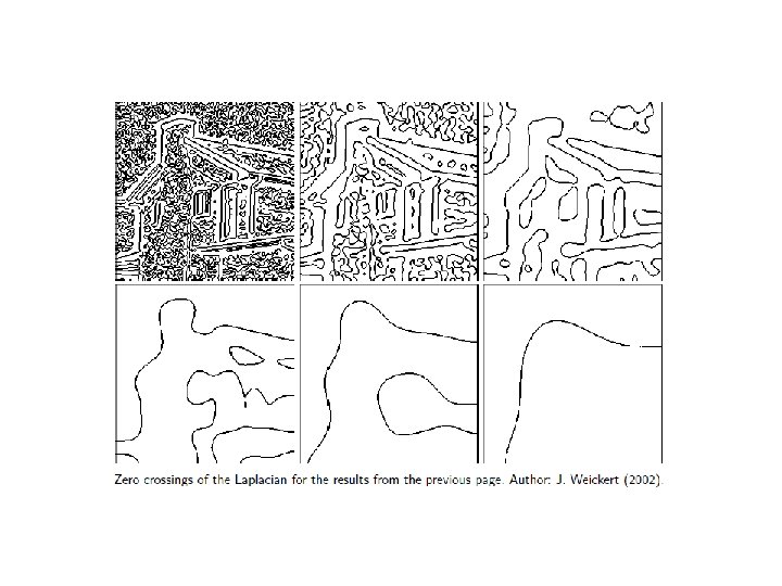
Edge Detection via 2 nd Order Derivatives • Compute Laplacian of Gaussian (Lo. G) – ∆u = uxx+uyy where u is a Gaussian smoothed image (u= Kσ*f). • Edges correspond to zero-crossings of the Lo. G ∆u.

Edge Detection via 2 nd Order Derivatives • Advantages – Single pixel thick edges that form closed contours – No additional parameters besides σ. • Disadvantages – 2 nd order derivatives are more sensitive to noise than 1 st order derivatives. – Can give false edges.