CPE 619 2 kp Factorial Design Aleksandar Milenkovi

CPE 619 2 k-p Factorial Design Aleksandar Milenković The La. CASA Laboratory Electrical and Computer Engineering Department The University of Alabama in Huntsville http: //www. ece. uah. edu/~milenka http: //www. ece. uah. edu/~lacasa

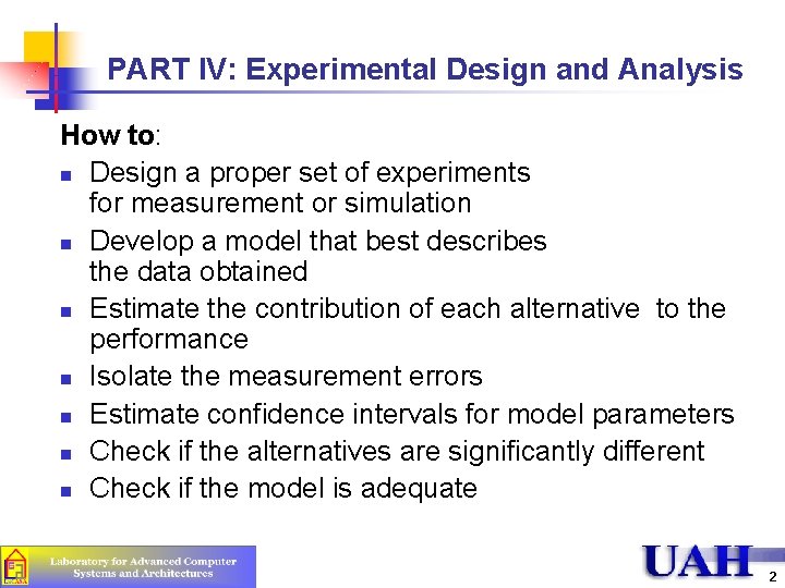
PART IV: Experimental Design and Analysis How to: n Design a proper set of experiments for measurement or simulation n Develop a model that best describes the data obtained n Estimate the contribution of each alternative to the performance n Isolate the measurement errors n Estimate confidence intervals for model parameters n Check if the alternatives are significantly different n Check if the model is adequate 2

Introduction n n n 2 k-p Fractional Factorial Designs Sign Table for a 2 k-p Design Confounding Other Fractional Factorial Designs Algebra of Confounding Design Resolution 3

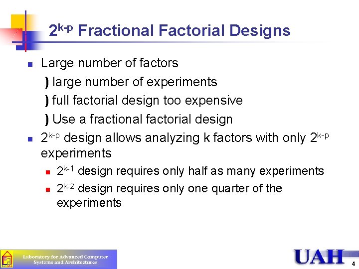
2 k-p Fractional Factorial Designs n n Large number of factors ) large number of experiments ) full factorial design too expensive ) Use a fractional factorial design 2 k-p design allows analyzing k factors with only 2 k-p experiments n n 2 k-1 design requires only half as many experiments 2 k-2 design requires only one quarter of the experiments 4

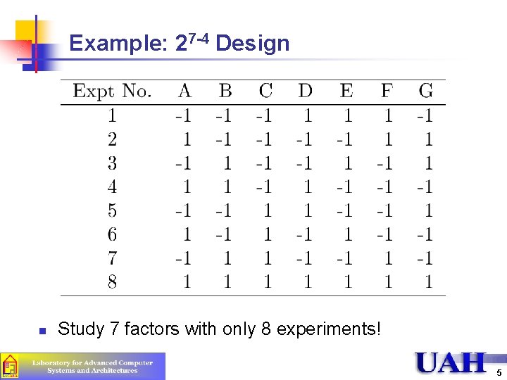
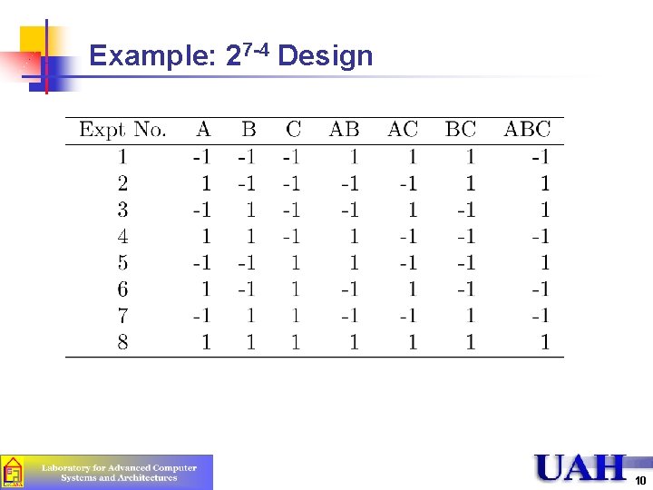
Example: 27 -4 Design n Study 7 factors with only 8 experiments! 5

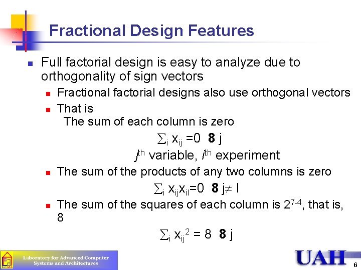
Fractional Design Features n Full factorial design is easy to analyze due to orthogonality of sign vectors n n Fractional factorial designs also use orthogonal vectors That is The sum of each column is zero åi xij =0 8 j jth variable, ith experiment n The sum of the products of any two columns is zero åi xijxil=0 8 j¹ l n The sum of the squares of each column is 27 -4, that is, 8 åi xij 2 = 8 8 j 6

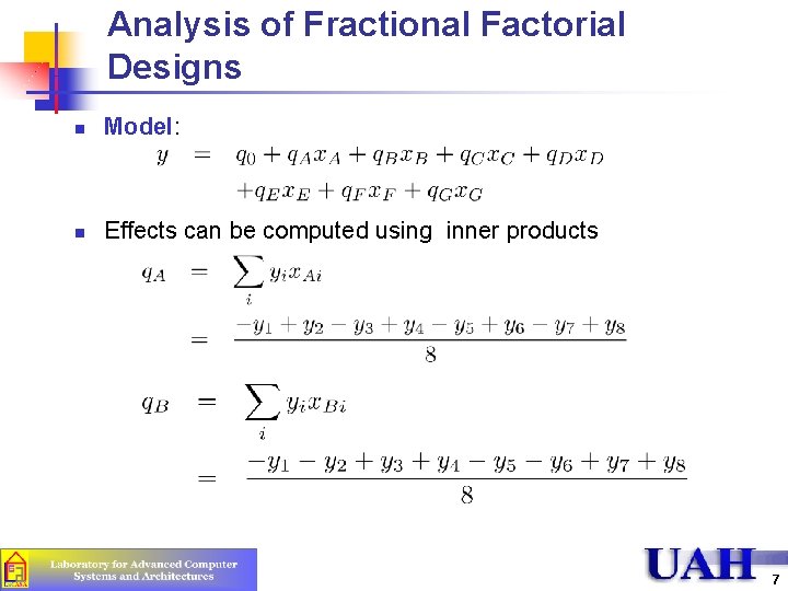
Analysis of Fractional Factorial Designs n Model: n Effects can be computed using inner products 7

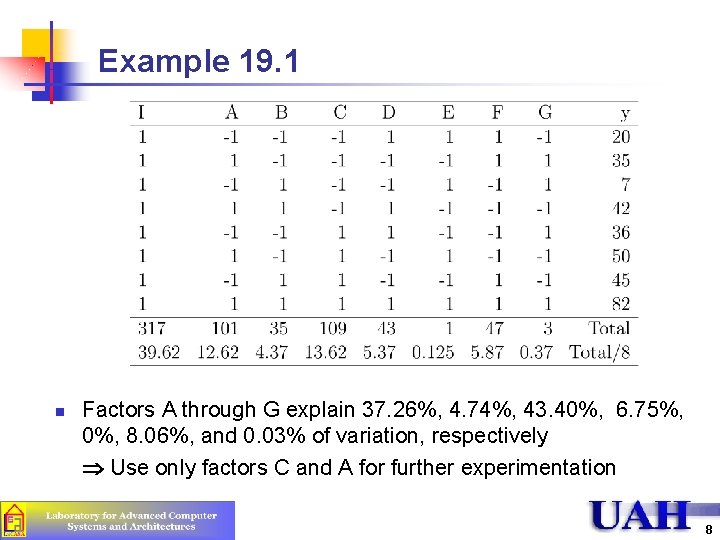
Example 19. 1 n Factors A through G explain 37. 26%, 4. 74%, 43. 40%, 6. 75%, 0%, 8. 06%, and 0. 03% of variation, respectively Use only factors C and A for further experimentation 8

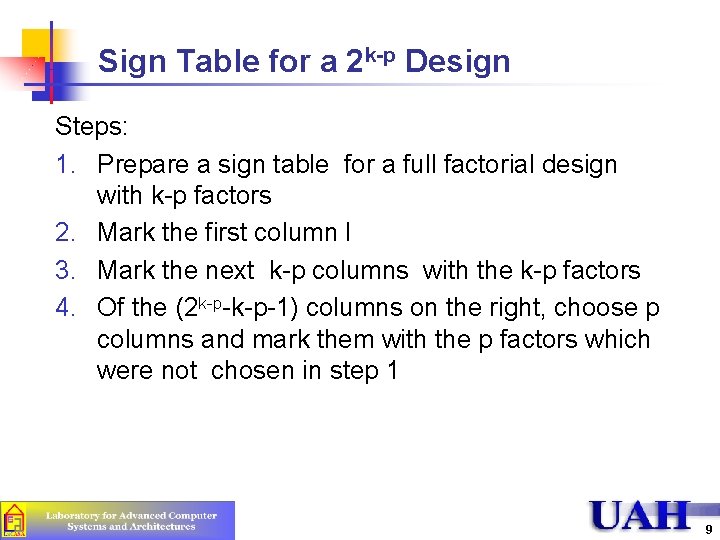
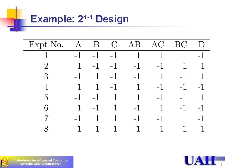
Sign Table for a 2 k-p Design Steps: 1. Prepare a sign table for a full factorial design with k-p factors 2. Mark the first column I 3. Mark the next k-p columns with the k-p factors 4. Of the (2 k-p-1) columns on the right, choose p columns and mark them with the p factors which were not chosen in step 1 9

Example: 27 -4 Design 10

Example: 24 -1 Design 11

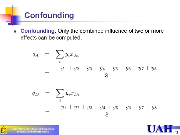
Confounding n Confounding: Only the combined influence of two or more effects can be computed. 12

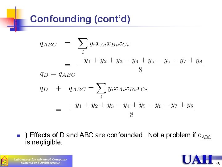
Confounding (cont’d) n ) Effects of D and ABC are confounded. Not a problem if q. ABC is negligible. 13

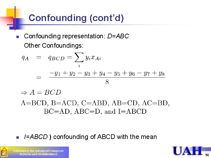
Confounding (cont’d) n n Confounding representation: D=ABC Other Confoundings: I=ABCD ) confounding of ABCD with the mean 14

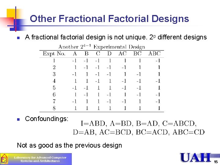
Other Fractional Factorial Designs n A fractional factorial design is not unique. 2 p different designs n Confoundings: Not as good as the previous design 15

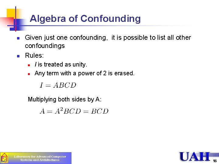
Algebra of Confounding n n Given just one confounding, it is possible to list all other confoundings Rules: n n I is treated as unity. Any term with a power of 2 is erased. Multiplying both sides by A: 16

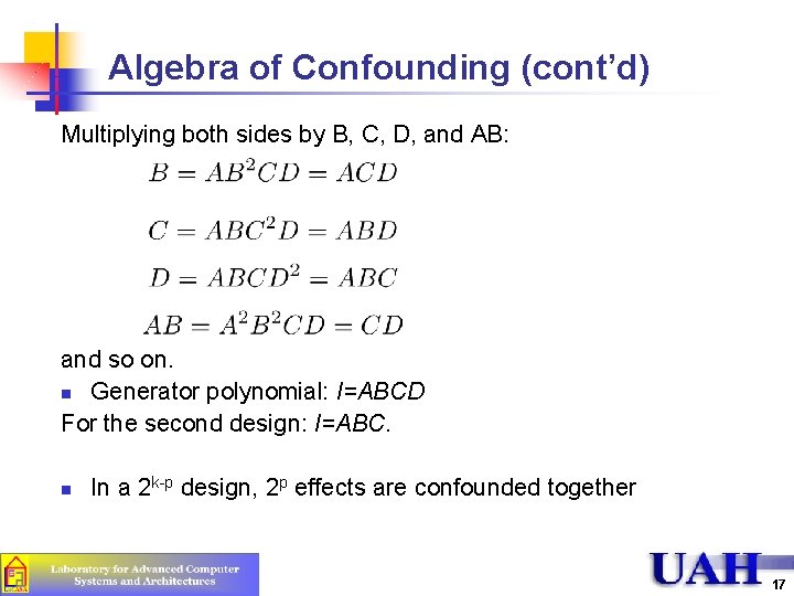
Algebra of Confounding (cont’d) Multiplying both sides by B, C, D, and AB: and so on. n Generator polynomial: I=ABCD For the second design: I=ABC. n In a 2 k-p design, 2 p effects are confounded together 17

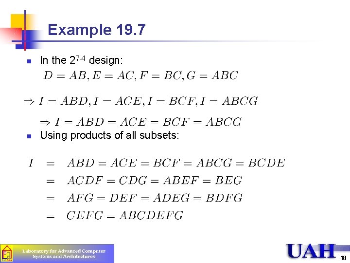
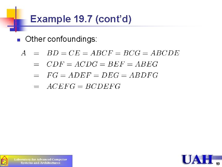
Example 19. 7 n In the 27 -4 design: n Using products of all subsets: 18

Example 19. 7 (cont’d) n Other confoundings: 19

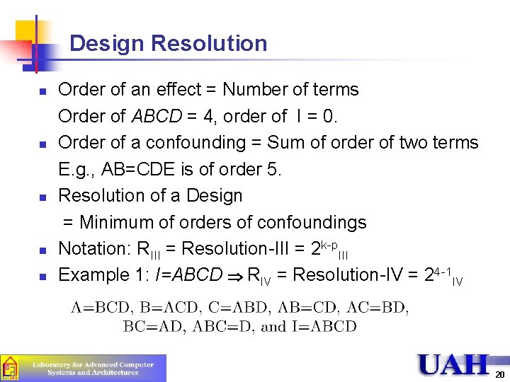
Design Resolution n n Order of an effect = Number of terms Order of ABCD = 4, order of I = 0. Order of a confounding = Sum of order of two terms E. g. , AB=CDE is of order 5. Resolution of a Design = Minimum of orders of confoundings Notation: RIII = Resolution-III = 2 k-p. III Example 1: I=ABCD RIV = Resolution-IV = 24 -1 IV 20

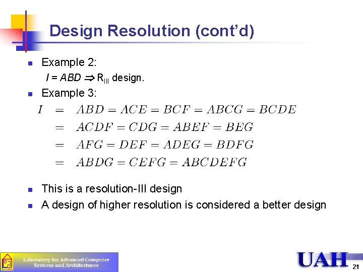
Design Resolution (cont’d) n n Example 2: I = ABD RIII design. Example 3: This is a resolution-III design A design of higher resolution is considered a better design 21

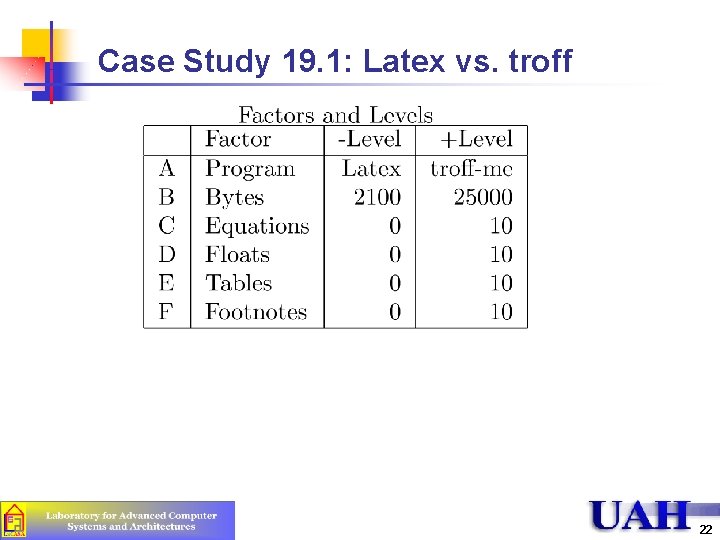
Case Study 19. 1: Latex vs. troff 22

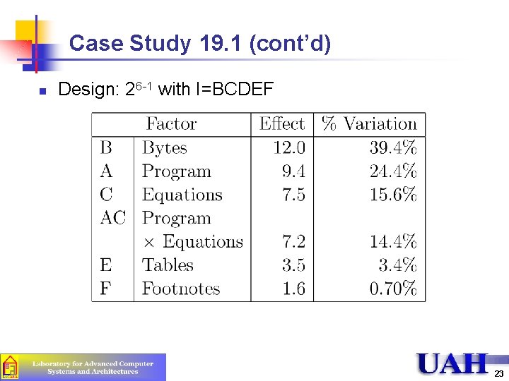
Case Study 19. 1 (cont’d) n Design: 26 -1 with I=BCDEF 23

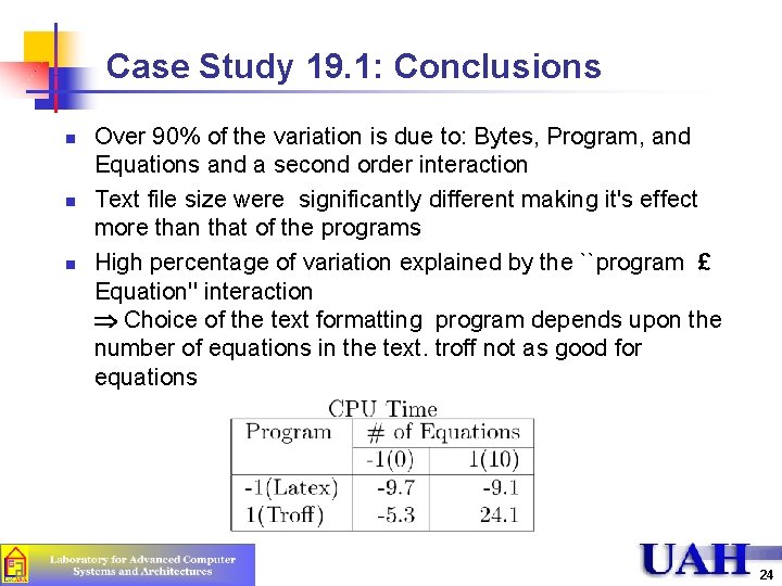
Case Study 19. 1: Conclusions n n n Over 90% of the variation is due to: Bytes, Program, and Equations and a second order interaction Text file size were significantly different making it's effect more than that of the programs High percentage of variation explained by the ``program £ Equation'' interaction Choice of the text formatting program depends upon the number of equations in the text. troff not as good for equations 24

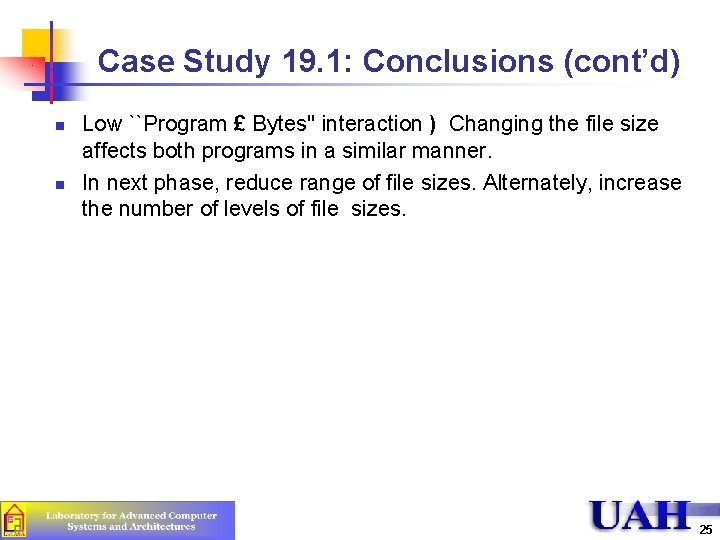
Case Study 19. 1: Conclusions (cont’d) n n Low ``Program £ Bytes'' interaction ) Changing the file size affects both programs in a similar manner. In next phase, reduce range of file sizes. Alternately, increase the number of levels of file sizes. 25

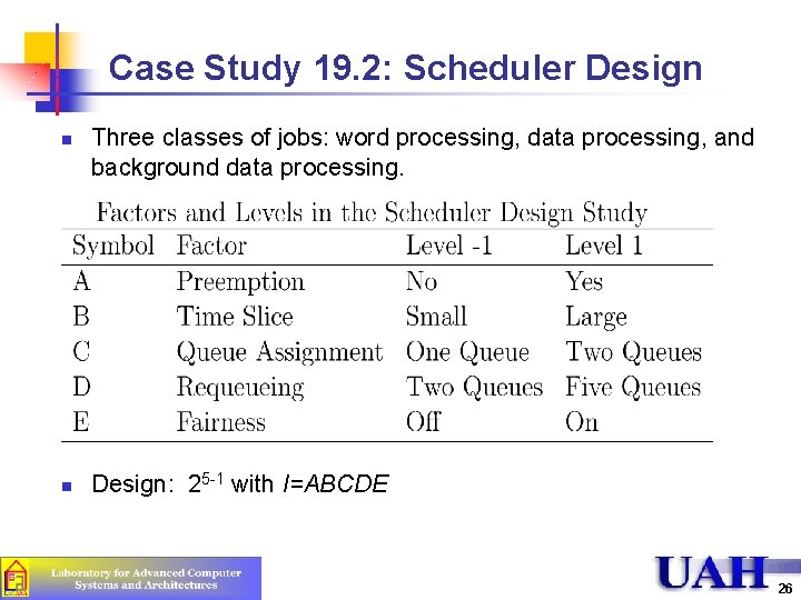
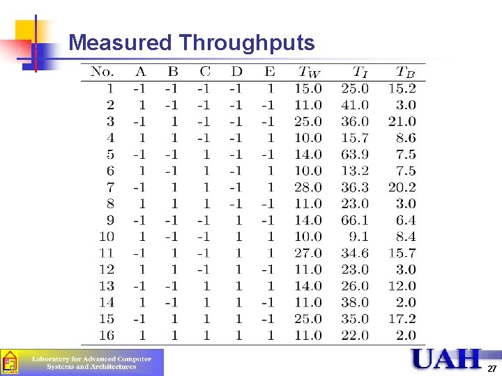
Case Study 19. 2: Scheduler Design n n Three classes of jobs: word processing, data processing, and background data processing. Design: 25 -1 with I=ABCDE 26

Measured Throughputs 27

Effects and Variation Explained 28

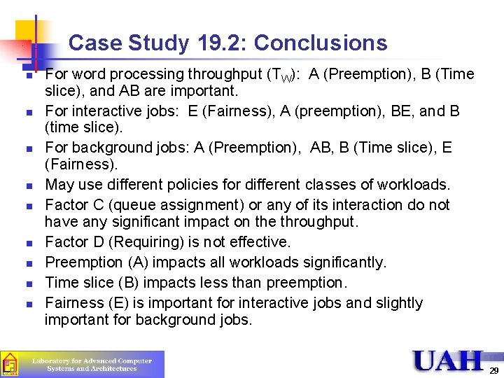
Case Study 19. 2: Conclusions n n n n n For word processing throughput (TW): A (Preemption), B (Time slice), and AB are important. For interactive jobs: E (Fairness), A (preemption), BE, and B (time slice). For background jobs: A (Preemption), AB, B (Time slice), E (Fairness). May use different policies for different classes of workloads. Factor C (queue assignment) or any of its interaction do not have any significant impact on the throughput. Factor D (Requiring) is not effective. Preemption (A) impacts all workloads significantly. Time slice (B) impacts less than preemption. Fairness (E) is important for interactive jobs and slightly important for background jobs. 29

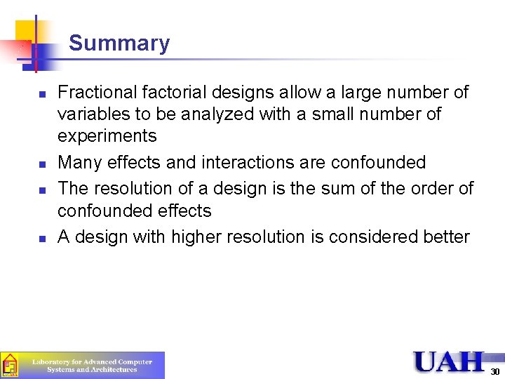
Summary n n Fractional factorial designs allow a large number of variables to be analyzed with a small number of experiments Many effects and interactions are confounded The resolution of a design is the sum of the order of confounded effects A design with higher resolution is considered better 30

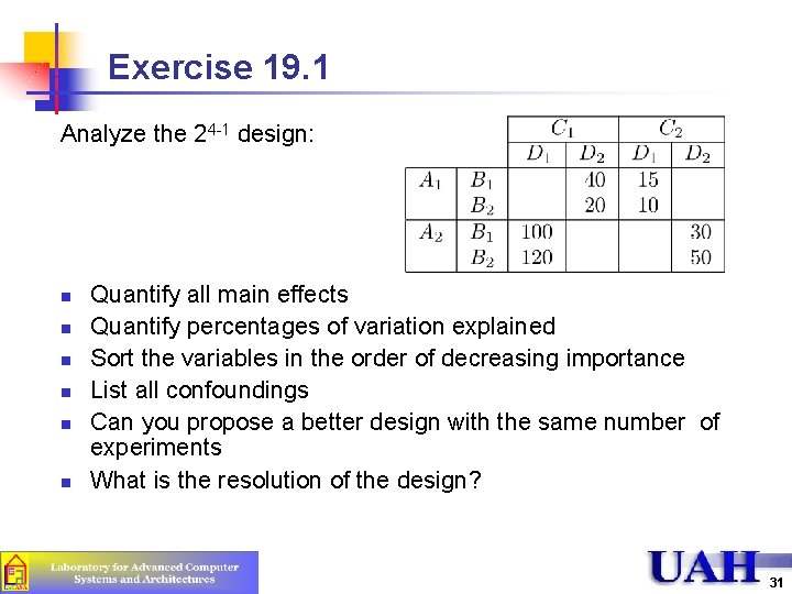
Exercise 19. 1 Analyze the 24 -1 design: n n n Quantify all main effects Quantify percentages of variation explained Sort the variables in the order of decreasing importance List all confoundings Can you propose a better design with the same number of experiments What is the resolution of the design? 31

Exercise 19. 2 Is it possible to have a 24 -1 III design? a 24 -1 II design? 241 design? If yes, give an example. IV 32

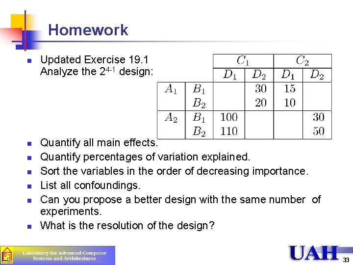
Homework n n n n Updated Exercise 19. 1 Analyze the 24 -1 design: Quantify all main effects. Quantify percentages of variation explained. Sort the variables in the order of decreasing importance. List all confoundings. Can you propose a better design with the same number of experiments. What is the resolution of the design? 33