https xkcd com619 CRISPDM COMP 309 Data preparation

https: //xkcd. com/619/

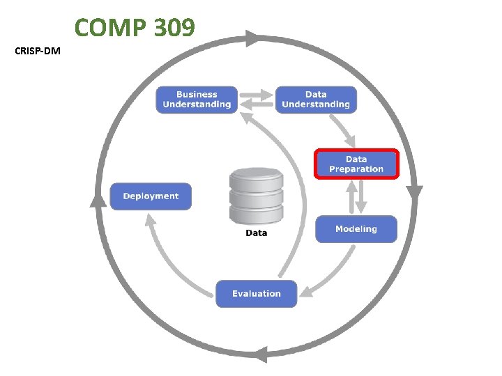
CRISP-DM COMP 309

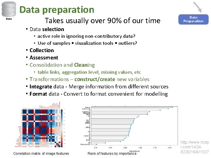
Data preparation Takes usually over 90% of our time • Data selection • active role in ignoring non-contributory data? • Use of samples • visualization tools • outliers? • Collection • Assessment • Consolidation and Cleaning • table links, aggregation level, missing values, etc • Transformations – construct/create new variables • Integrate data - Merge information from different sources • Format data - Convert to format convenient for modelling Correlation matrix of image features Rank of features by importance http: //www. mdp i. com/14248220/18/4/1027

Feature Selection, Construction and Extraction Amazon. com (Not recommended reading!)

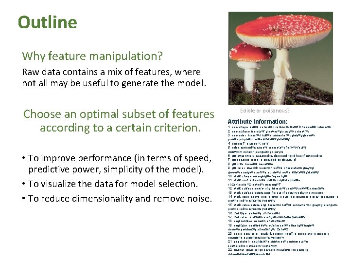
Outline Why feature manipulation? Raw data contains a mix of features, where not all may be useful to generate the model. Choose an optimal subset of features according to a certain criterion. • To improve performance (in terms of speed, predictive power, simplicity of the model). • To visualize the data for model selection. • To reduce dimensionality and remove noise. Edible or poisonous? Attribute Information: 1. cap-shape: bell=b, conical=c, convex=x, flat=f, knobbed=k, sunken=s 2. cap-surface: fibrous=f, grooves=g, scaly=y, smooth=s 3. cap-color: brown=n, buff=b, cinnamon=c, gray=g, green=r, pink=p, purple=u, red=e, white=w, yellow=y 4. bruises? : bruises=t, no=f 5. odor: almond=a, anise=l, creosote=c, fishy=y, foul=f, musty=m, none=n, pungent=p, spicy=s 6. gill-attachment: attached=a, descending=d, free=f, notched=n 7. gill-spacing: close=c, crowded=w, distant=d 8. gill-size: broad=b, narrow=n 9. gill-color: black=k, brown=n, buff=b, chocolate=h, gray=g, green=r, orange=o, pink=p, purple=u, red=e, white=w, yellow=y 10. stalk-shape: enlarging=e, tapering=t 11. stalk-root: bulbous=b, club=c, cup=u, equal=e, rhizomorphs=z, rooted=r, missing=? 12. stalk-surface-above-ring: fibrous=f, scaly=y, silky=k, smooth=s 13. stalk-surface-below-ring: fibrous=f, scaly=y, silky=k, smooth=s 14. stalk-color-above-ring: brown=n, buff=b, cinnamon=c, gray=g, orange=o, pink=p, red=e, white=w, yellow=y 15. stalk-color-below-ring: brown=n, buff=b, cinnamon=c, gray=g, orange=o, pink=p, red=e, white=w, yellow=y 16. veil-type: partial=p, universal=u 17. veil-color: brown=n, orange=o, white=w, yellow=y 18. ring-number: none=n, one=o, two=t 19. ring-type: cobwebby=c, evanescent=e, flaring=f, large=l, none=n, pendant=p, sheathing=s, zone=z 20. spore-print-color: black=k, brown=n, buff=b, chocolate=h, green=r, orange=o, purple=u, white=w, yellow=y 21. population: abundant=a, clustered=c, numerous=n, scattered=s, several=v, solitary=y 22. habitat: grasses=g, leaves=l, meadows=m, paths=p, urban=u, waste=w, woods=d

Feature engineering Can be split into dimensionality reduction and dimensionality changing techniques: Dimensionality reduction: 1) Feature extraction methods apply a transformation on the original feature vector to reduce its dimension from d to m. 2) Feature selection methods select a small subset of original features. Dimensionality changing: 3) Feature construction is a process that discovers missing information about the relationships between features and augments the space of features by inferring or creating additional features. The original features may or may not be replaced, hence the dimensionality can change in many ways https: //www. tik. ee. ethz. ch/file/f 9 ed 2 d 0 d 19540 a 6 a 287 d 4 b 6 f 0 a 24 da 6 0/feature. Selection_Extraction. pdf

Feature extraction Transform the original feature vector to reduce its dimension from d to m. https: //www. tik. ee. ethz. ch/file/f 9 ed 2 d 0 d 19540 a 6 a 287 d 4 b 6 f 0 a 24 da 6 0/feature. Selection_Extraction. pdf

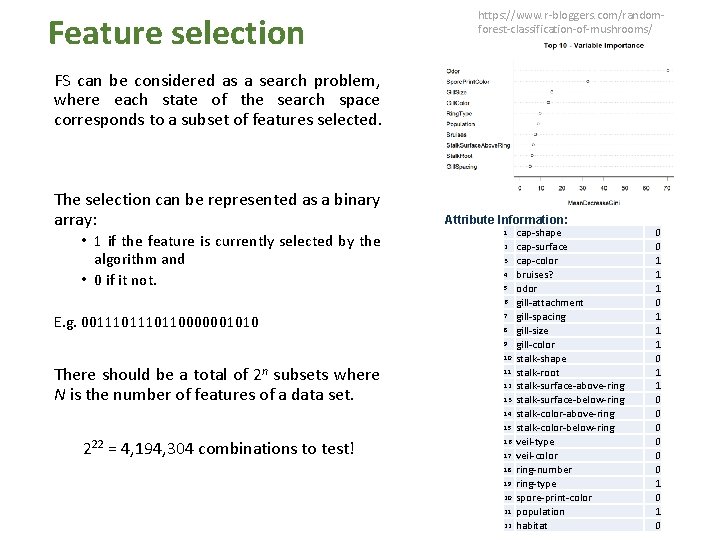
Feature selection https: //www. r-bloggers. com/randomforest-classification-of-mushrooms/ FS can be considered as a search problem, where each state of the search space corresponds to a subset of features selected. The selection can be represented as a binary array: • 1 if the feature is currently selected by the algorithm and • 0 if it not. Attribute Information: 1 2 3 4 5 6 E. g. 001110110000001010 7 8 9 10 There should be a total of 2 n subsets where N is the number of features of a data set. 11 12 13 14 15 222 = 4, 194, 304 combinations to test! 16 17 18 19 20 21 22 cap-shape cap-surface cap-color bruises? odor gill-attachment gill-spacing gill-size gill-color stalk-shape stalk-root stalk-surface-above-ring stalk-surface-below-ring stalk-color-above-ring stalk-color-below-ring veil-type veil-color ring-number ring-type spore-print-color population habitat 0 0 1 1 1 0 0 0 1 0

Feature selection Useful for high dimensional data, such as genomic DNA and text documents. Methods • Univariate (Considers a feature independently of others) • Pearson correlation coefficient • Chi-square • Signal to noise ratio • F-score And more such as mutual information, Relief • Multivariate (Considers all features simultaneously) • Dimensionality reduction algorithms • Linear classifiers such as support vector machine • Recursive feature elimination

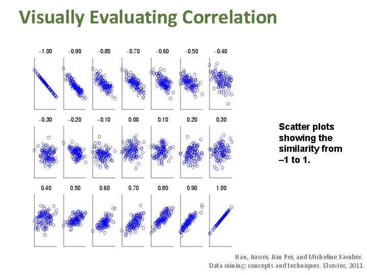
Visually Evaluating Correlation Scatter plots showing the similarity from – 1 to 1. Han, Jiawei, Jian Pei, and Micheline Kamber. Data mining: concepts and techniques. Elsevier, 2011.

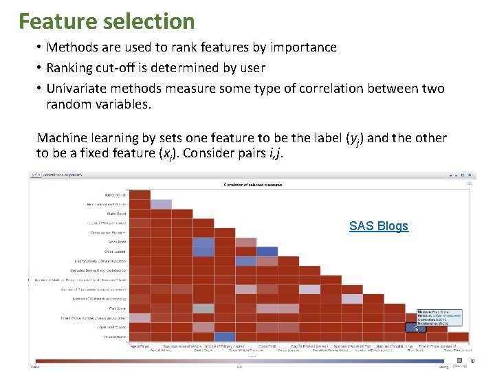
Feature selection • Methods are used to rank features by importance • Ranking cut-off is determined by user • Univariate methods measure some type of correlation between two random variables. Machine learning by sets one feature to be the label (yj) and the other to be a fixed feature (xi). Consider pairs i, j. SAS Blogs

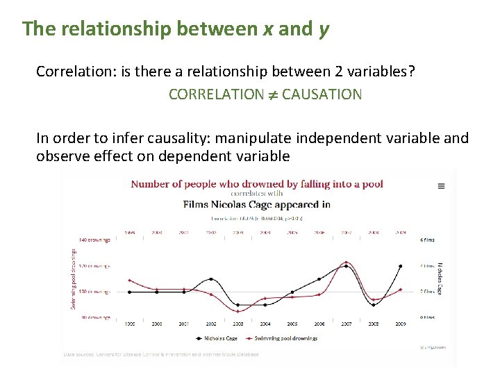
The relationship between x and y Correlation: is there a relationship between 2 variables? CORRELATION CAUSATION In order to infer causality: manipulate independent variable and observe effect on dependent variable

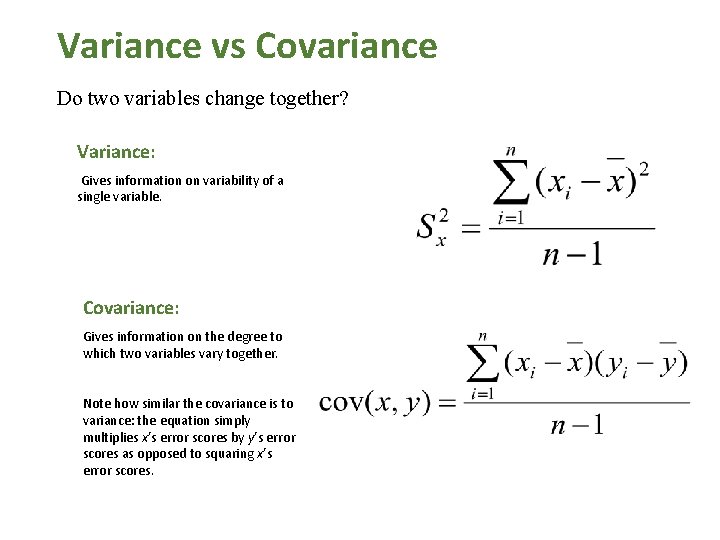
Variance vs Covariance Do two variables change together? Variance: Gives information on variability of a single variable. Covariance: Gives information on the degree to which two variables vary together. Note how similar the covariance is to variance: the equation simply multiplies x’s error scores by y’s error scores as opposed to squaring x’s error scores.

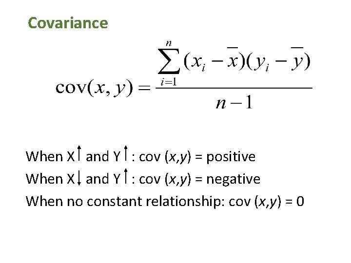
Covariance When X and Y : cov (x, y) = positive When X and Y : cov (x, y) = negative When no constant relationship: cov (x, y) = 0

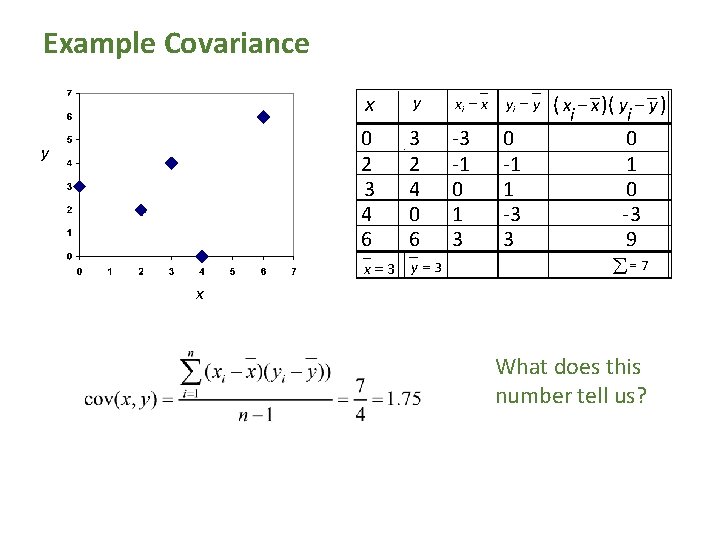
Example Covariance y x x y 0 2 3 4 6 3 2 4 0 6 x=3 xi - x -3 -1 0 1 3 y = 3 yi - y 0 -1 1 -3 3 ( xi - x )( yi - y ) 0 1 0 -3 9 å= 7 What does this number tell us?

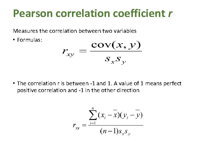
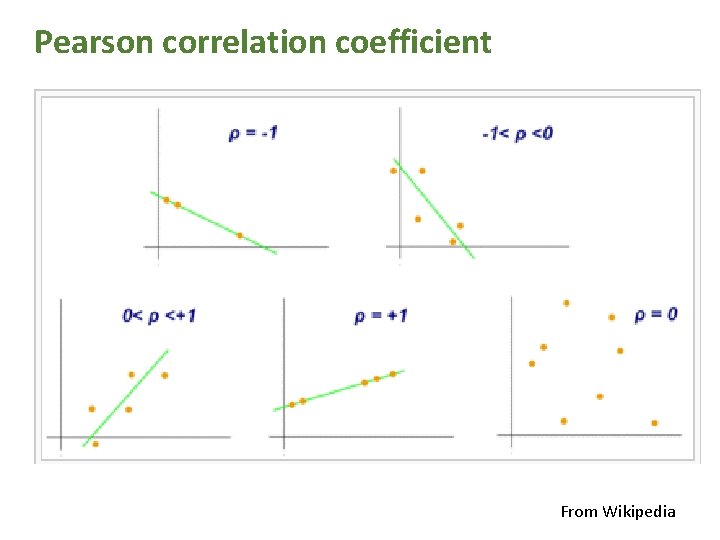
Pearson correlation coefficient r Measures the correlation between two variables • Formulas: • The correlation r is between -1 and 1. A value of 1 means perfect positive correlation and -1 in the other direction

Pearson correlation coefficient From Wikipedia

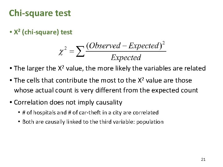
Chi-square test • Χ 2 (chi-square) test • The larger the Χ 2 value, the more likely the variables are related • The cells that contribute the most to the Χ 2 value are those whose actual count is very different from the expected count • Correlation does not imply causality • # of hospitals and # of car-theft in a city are correlated • Both are causally linked to the third variable: population 21

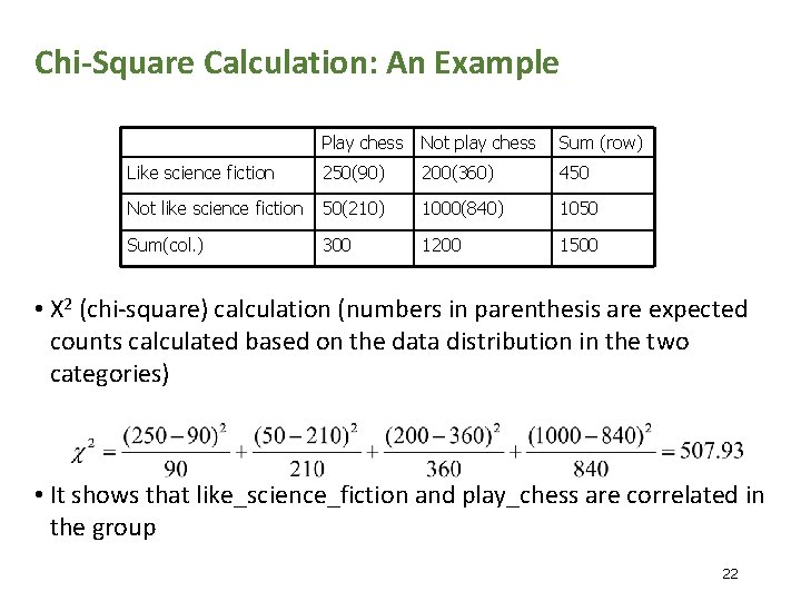
Chi-Square Calculation: An Example Play chess Not play chess Sum (row) Like science fiction 250(90) 200(360) 450 Not like science fiction 50(210) 1000(840) 1050 Sum(col. ) 300 1200 1500 • Χ 2 (chi-square) calculation (numbers in parenthesis are expected counts calculated based on the data distribution in the two categories) • It shows that like_science_fiction and play_chess are correlated in the group 22

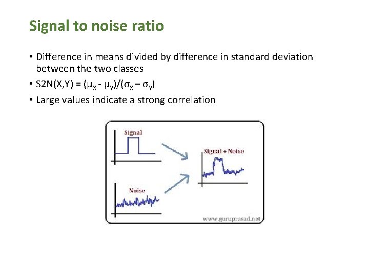
Signal to noise ratio • Difference in means divided by difference in standard deviation between the two classes • S 2 N(X, Y) = (μX - μY)/(σX – σY) • Large values indicate a strong correlation

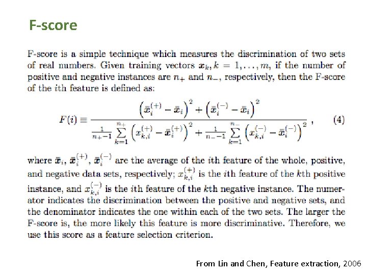
F-score From Lin and Chen, Feature extraction, 2006

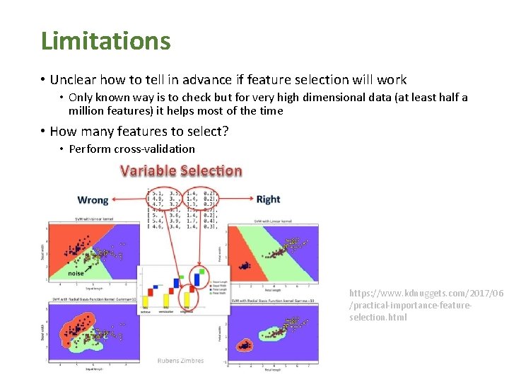
Limitations • Unclear how to tell in advance if feature selection will work • Only known way is to check but for very high dimensional data (at least half a million features) it helps most of the time • How many features to select? • Perform cross-validation https: //www. kdnuggets. com/2017/06 /practical-importance-featureselection. html

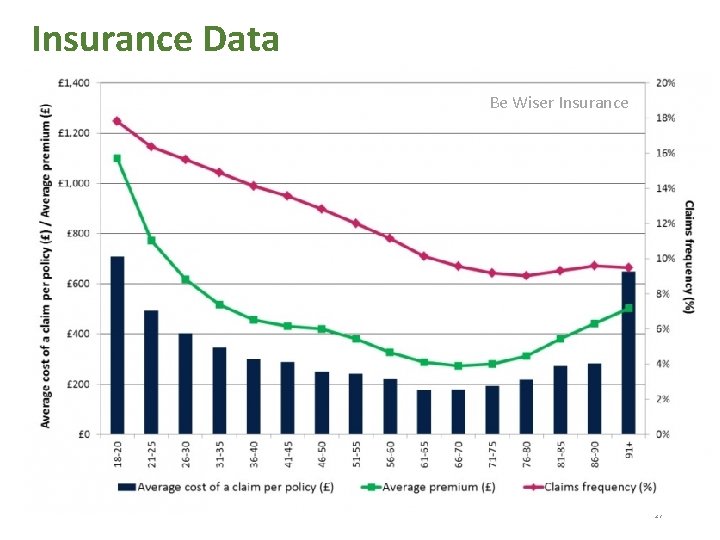
Insurance Data • Price rise from $2300 a year to $12, 843 • The company will roll out fully riskbased assessments for flooding, erosion, storm and other identifiable risks. • "Our new approach removes much of these cross-subsidisation in house insurance premiums, meaning what customers pay will more accurately reflect the cost of providing cover for their individual property. ” • NZbrokers service manager Simon Moss said Tower appeared to be disengaging from some regions. It was possible to assess risk on a house by house basis with all the data available nowadays, he said. 26

Insurance Data Be Wiser Insurance 27

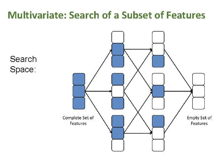
Multivariate: Search of a Subset of Features Search Space:

Multivariate: Subset of Features • Search Directions: • Sequential Forward Generation (SFG): It starts with an empty set of features S. As the search starts, features are added into S according to some criterion that distinguish the best feature from the others. S grows until it reaches a full set of original features. The stopping criteria can be a threshold for the number of relevant features m or simply the generation of all possible subsets in brute force mode. • Sequential Backward Generation (SBG): It starts with a full set of features and , iteratively, they are removed one at a time. Here, the criterion must point out the worst or least important feature. By the end, the subset is only composed of a unique feature, which is considered to be the most informative of the whole set. As in the previous case, different stopping criteria can be used.

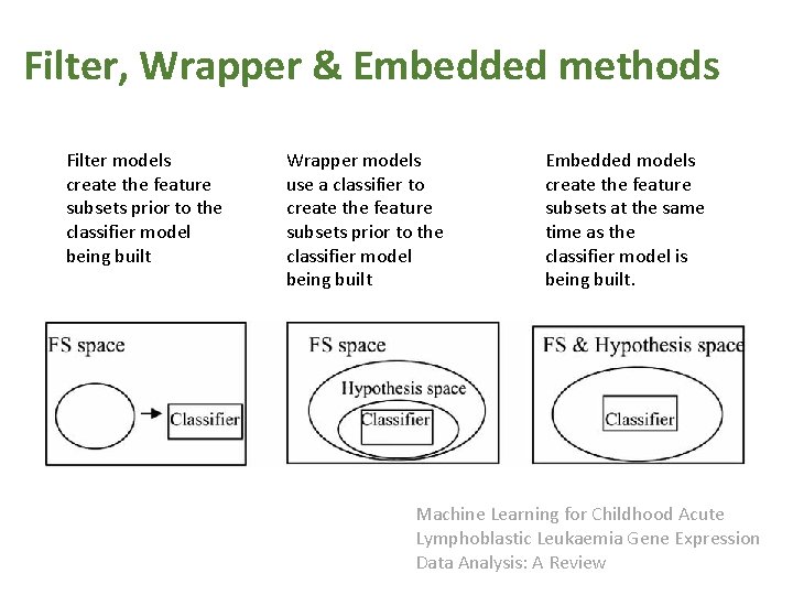
Filter, Wrapper & Embedded methods Filter models create the feature subsets prior to the classifier model being built Wrapper models use a classifier to create the feature subsets prior to the classifier model being built Embedded models create the feature subsets at the same time as the classifier model is being built. Machine Learning for Childhood Acute Lymphoblastic Leukaemia Gene Expression Data Analysis: A Review